


 Inglés (pdf)
 Articulo en XML
 Referencias del artículo
 Enviar articulo por email
 Citado por SciELO
  Similares en
SciELO
Similares en
SciELO 
 Permalink
1. Introduction
Nowadays Fault Tolerant capabilities are increasingly important for control systems. Operation interruptions for applications such as energy distribution systems are very expensive as can be seen in works like Linares and Rey (2013). For induction motors is almost mandatory to be fault tolerant due a large variety of applications are based on them (Fernandez-Cavero et al. (2015)). Fault tolerant capabilities not only saves maintenance cost but also increase controlled system’s safety. As pointed out in Gaoet al. (2015a), other applications such as aero engines, vehicle dynamics, chemical processes among others are increasing demand for fault tolerant control strategies.
The fault diagnosis problem can be addressed using hardware or analytical redundancy. Since 1980s analytical redundancy has gained high interests because it saves costs and allows to minimize space (Gao et al. (2015b)). With a trustfully mathematical plant’s model that includes fault effects is possible to design a controller able to properly work not only in normal case operation but also if failures occur.
It can be seen in Wang and Jiang (2017) that a fault tolerant MPC controller is implemented, where the faults are treated as disturbances. Then the controller is designed to be robust against disturbance.
Another approach based in the unknown input observer can be seen in (Noura et al., 2009, p. 34-35). The compensation schema is based in an additive control law that is calculated employing the residual signals and the controlled system’s model.
Also, in Seron and Don (2015) a compensation for LPV systems is proposed wherein the controller gains are updated according to varying parameters and the residual signals.
As mentioned in Khan et al. (2017), DMC controller offers a superior performance when compared to PID controller but DMC need to show high reliability in order to replace them in the industry. In the interest of improving MPC robustness, a new fault tolerant control method is developed and tested in this work, in which a first order derivative is used to detect and quantify a fault earlier. This allows to tune the dynamic matrices of the MPC controller accordingly to the magnitude of the failure, making a more robust system. To accomplish this, it was necessary to build a non-linear model for the heat exchanger in order to build a reliable residual generator. Experimental results showed that this approach improved the system’s robustness by shortening the recovering time. Despite of this improvement, it was also observed that an additive law inspired in (Noura et al., 2009, p. 34-36) is even superior when it comes to reducing fault impact in the controlled variable.
2. The Heater Cooler Model Development
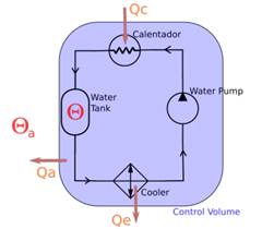
The heater-Cooler system used in this work is shown in Figure 1. This is an educational control system from the manufacturer LabVolt (model: 6090), available in the control and automation laboratory. This training system is used for experiments such as pressure, liquid level, flow and heat transfer control. This system comprises a water pump which establishes a constant flow rate, two temperature sensors, an electric heater and cooler fans. The sensor measures ambient temperature and the water temperature in the tank, which is the controlled variable (see Figure 1). Hence this system comprises two inputs and one output. The water keeps recirculating indefinitely and its mass remains constant over time.

2.1. Dynamic Model Derivation
A control volume, to apply energy conservation law, is chosen that it contains the whole system as depicted in Figure 2. This approach is feasible given that the temperature difference at any point in the water path is less than 0.5 K. For practical purposes the temperature in the water tank is assumed as the entire system’s temperature. In Figure 2 is shown that the only heat gain Qc is due to the electric heater whereas heat loss is due to cooler fans (Qe) and the gradient temperature between water and outside temperature (Qa). the systems dynamic model must to meet energy conservation law, that is an equation in the form Qt = Qc − Qa − Qe.
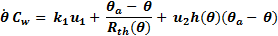
The power dissipated in the electric heater is given by Pc= IV. To adjusts the amount of energy transformed into heat, pulse width modulation is applied to the heater input voltage, that is AC grid voltage. The actuator control signal sets the time within the grid period that the voltage is applied to the resistance, ranging from 0% at 0 Volts to 100% at 5 Volts. When the full AC period is set, the heater nominal power is 950 W. Then the heat gain Qc, due to the electric heater, can be expressed in the form k 1*u 1, where k 1 = 950W/5. This can be seen expressed in Equation 1, that is the complete system’s dynamic model.
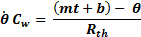
Fourier heat conduction law states that the amount of heat flux transferred by thermal conduction is proportional to the temperature difference between the (Wang et al., 2007, p. 19). Given that the heater-cooler system is not anisotropic medium and have a complex geometry, it is necessary to use the concept of overall thermal resistivity (Thulukkanam, 2013, p. 27-31) to model the heat loss from the recirculating water to the outside. This can be seen next to k1*u1 in equation 1, where Θa is the outside overall temperature and Θ is the water temperature measured at the tank. Thermal resistivity is represented as Rth(Θ) and it was found that this parameter is highly Dependent on water temperature. The calculations to compute this parameter are explained in the next section.
 (1)
(1)
The cooler is made of fans to extract heat by forced convection. This implies that is not possible to reach a temperature below the environment. This also implies that the heat loss must be also proportional to the temperature difference between the water and the outside. Also, it must to be proportional to the fan’s angular speed that is controlled by input signal u
1, that also ranges from 0 to 5. The convection constant, represented in Equation 1 by h(Θ) is related to the material properties and geometries involved in the heat transfer caused by the forced convection. It can be seen that if the temperature difference is zero, the heat flux is also zero regardless the chosen value for u
2. The left side in Equation 1 is the net heat flux into the system. According to classical thermodynamics, the heat change experienced by an object is given by Q = C∆Θ where C is the thermal capacity. Then a differential heat change is given by dQ = CdΘ. Dividing both sides by dt, the heat flux is obtained. Hence the net heat flux caused by a change in temperature is given by  = C
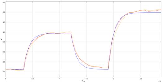
= C as expressed in Equation 1. The heater-cooler system is clearly a nonlinear system. The latter can be seen also in the experimental open loop curves presented in Figure 3 where the rise and fall times are different. This can be explained by the thermal resistivity which increases as the water temperature is decreasing, as a result, the system is cooled down slower over time.
2.2 Overall Thermal Resistivity Calculation
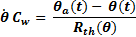
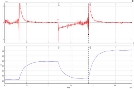
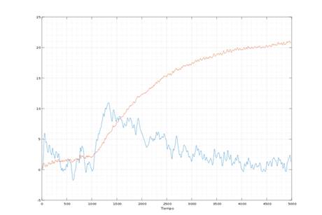
The thermal resistivity was calculated using heat-cooling experiments as depicted in Figure 4 (downside curve). In those experiments the control input u 2 was set to 0, hence the heat flux related to the cooler is canceled. To estimate the thermal resistivity, the water is heated at constant heat flux by the electric heater. When steady state is reached, the heater flux is canceled by setting u 1 = 0. Hence the only heat flux is due to temperature gradient between the system and the environment. That is, during the time interval within the cursors in the downside graph at Figure 4, the water’s temperature is governed by the Equation 2. From this equation thermal resistivity can be obtain as expressed in Equation 3, which is depicted in the upside curve in Figure 4. This upside graph clearly shows that thermal resistivity increases as the system is cooling down. However, direct use of Equation 3 did not lead to an accurate model due to the high uncertainty. To use such direct method is necessary to use high accuracy and resolution temperature sensors.
 (2)
(2)
 (3)
(3)
To obtain better results, it was necessary to solve the thermal resistivity using minimum mean square error method. For this purpose, the experiment data were segmented in small enough segments such that the outside temperature Θa could be approximated by a linear curve and thermal resistivity could be considered as constant. This leads to Equation 4, where ambient temperature was replaced by a linear function. To simplify the equation, thermal capacity and thermal resistivity are mixed in a single parameter as shown in Equation 5. Considering that Equation 4 is only accurate for a very small segment during the natural cooldown period, an analytical solution can be obtained for such segment that is presented in Equation 6. For this equation should exist a value for R such that the small enough selected segment is well fitted in the minimal square sense. Using temperature and time vectors obtained from experiments, an optimal value for R can be calculated for a given segment. Considering the above, a Matlab algorithm was developed. The algorithm was responsible to build a set of small enough segments. For each segment a linear approximation for ambient temperature was computed. Afterwards, for each segment, constant R was solved according to Equation 6 and square error minimization principle. As output, a set of values for R was obtained.
 (4)
(4)
 (5)
(5)
 (6)
(6)
3. MPC Controller Implementation
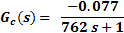
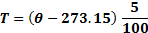
The implemented MPC controller is based on DMC strategy which require the plant models as a step response vector. Therefore, it was necessary to develop an approximate linearized model, since the model presented in 1 even though more precise it is not linear. A first order transfer function parametric approximation was made using the experimental data. In the Equation 7 a transfer function is shown, which corresponds to the electric heater, and the Equation 8 represents the transfer function of the cooler. MPC controller’s input ranges from 0 to 5 where 0 corresponds to 273.15K and 5 to 373.15K, the maximum temperature value. To adjust the measured temperature to this range, the read temperature is scaled using Equation 9 Using transfer functions (Equations 9 and 10), a step response was built up as for the heater as for the cooler.
 (7)
(7)
 (8)
(8)
 (9)
(9)
It can be seen in the transfer functions that the cooler has the lowest settle time. Hence the sampling time is established as 20 s that is the 2.6% of the cooler’s transfer function time constant. The latter assure that the sampling time is enough to properly control heater and cooler dynamics. The control horizon was chosen empirically. The control and prediction horizon were incremented from test to test until not significant improvements were observed. The control horizon was settled at 5 samples while the prediction horizon was set as 30 samples. using Equation 10 is possible to calculate future outputs for a linear discrete system. Recall that a convolution between the step response and the input’s signal difference gives the systems response.
 (10)
(10)
The number of terms in Equation 10 depends on the number of outputs, inputs, control and prediction horizon size. The cost function used for the MPC is shown in Equation 11. By replacing y, from the Equation 10, into the cost function, a set of quadratic equations are obtained. In the cost function the first term is the difference between the reference signal and the measured temperature, that is the error signal. The second term is related to the control effort. By minimizing this function, a set of control values are obtained such that the error is minimized with the fewer energy consumption. In this case the cost function has 10 variables, 5 for the heater and 5 for the cooler. Khanet al. (2017).
 (11)
(11)
Solving ∇J = 0 to find the optimal control signals becomes into a quadratic programing problem. In order to use existing libraries to compute the solution for each iteration is necessary to adapt the cost function to the Equation12. To implement the on line quadratic optimization algorithm the approach proposed by Ferreau et al. (2014) was used.
 (12)
(12)
4. Fault Modelling
In this work, only faults related to the heater were considered. In particular, the studied fault was a reduction in the electric heater input voltage. Considering that the power consumed by the electric heater is Pc = IV, is feasible to model such fault as multiplicative. In Equation 13 a linearization around an equilibrium point is presented. The upper script ”*” in variables at Equation 13 denote that coordinate system is translated to equilibrium point. Based in superposition principle, the control action u 2 and the ambient temperature Θa are set to zero in order to obtain only the heater contribution to the systems dynamics. The resulting equation is shown in Equation 14, from which a transfer function representation is obtained (Equation 15). It can be seen in the transfer function that only the model gain is affected by the fault in the electric heater whereas the stabilization time remains unaltered.
 (13)
(13)
 (14)
(14)
 (15)
(15)
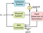
5. Fault Detection And Compensation
In Figure 5 is presented a simulation with the MPC controller and a 60% fault at t = 1500 s. It can be seen that even without fault compensation scheme, the controller is able to return to the reference temperature. In Figure 6 is depicted with continuous line the residual function which is almost 0 before the fault at t = 1500 s. When the fault appears, the residual behaves like a stable first order linear dynamic system. The residual signal in 6 reach steady state when the MPC controller is fully recovered from the fault.
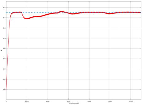
Fig. 5: Fault simulation with heater operating at 40% from its full nominal power. Controlled temperature is represented with the red continuous line. The reference signal is depicted blue dashed line.
The residual signal is computed as r(t) = Θ(t) − Θ sim (t), where Θ is the real measured temperature and Θ sim is the on-line calculated temperature through model exposed at Equation 1. Is clear that r(t) = 0 when the system is fault free in simulation, nevertheless this signal is not strictly zero as consequence of noise, model parameters uncertainty and not considered disturbances among others. To overcome this, a threshold must be established, using experimental data, such that residual stays inside.
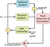
The threshold when operating in normal conditions. In this work, the threshold was set as ± 1.4K. Through the residual steady state value is possible to guess the faults magnitude. However, when this value is known it is too late for compensation. As pointed out in (Isermann, 2011, p. 25-26), using the residual derivative is possible to detect fault much faster. In this work a band pass filter was implemented to obtain an equivalent to residual derivative and also reduce the noise, which is a byproduct of the derivative operation. As can be appreciated in Figure 6, the blue dashed curve that is the result of applying a band pass filtering to the residual function. Once the fault occurrence is detected, the quantification process is done employing a peak detector and artificial neural networks (ANN). The ANN was trained using a dataset build entirely from simulation. Once the fault is measured, the compensation schema updates the gain in the MPC electric heater model. In Figure 7 is shown the proposed compensation schema.
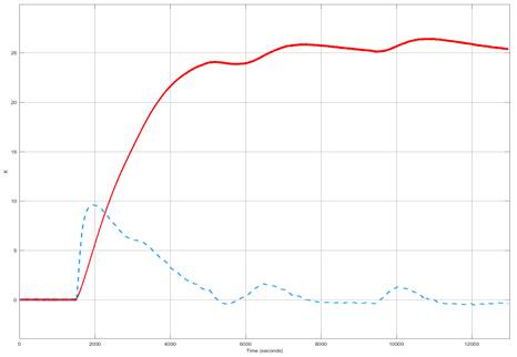
Fig. 6: Residual signal (represented by the continuous redline) and filtered residual signal (blue dashed line).
In Figure 8,Figure 9andFigure 10, experimental results are shown. A variac in series with the electric heater was used to induce faults into the system in a controlled manner. In Figure 8 the blue curve corresponds to a fault experiment without the compensation schema described above whereas green curve is the experiment with compensation schema. In both experiments fault was reproduced at the same relative time and magnitude.
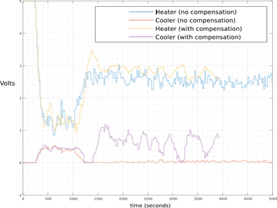
Due to the fault was induced in a controlled manner, the fault magnitude was known in experiments. The ANN retrieved accurate fault magnitude measures ranging from 10% to 120%. In the experiments was observed that updating MPC controller with the actual gain did not improved recovery time significantly. Other tests were made updating MPC heater model’s gain with lower values than the actual fault, as a result the MPC counter action was higher and an improvement can be seen in Figure 8. It can be seen in this case that the recovery time improves with the compensation scheme. But this is not a successful result due to it was obtained updating the MPC with a lower gain than the actual corresponding to the fault. The control signals are shown in Figure 10 for both cases, with the proposed compensation schema and without it. It can be seen that control signals for heater and cooler never surpass the range 0 − 5 neither of the two experiments. The IAE performance index was 5820,15 without any compensation and 4040,175 With the proposed compensation schema (using lower gain). The lack of success with the proposed method motivated another experiment with an additive compensation scheme, inspired by (Noura et al.,2009, p. 34-36) and depicted in Figure 11. In this case the residual derivative is used directly as the compensation signal. It can be seen that the residual derivative is always a single pulse that is proportional to the fault magnitude. During the experiments it was observed that using the right gain K (see Figure 11), The water’s temperature remains almost unaffected for a wide faults range. Even the fault occurrence cold not be noticed just by inspection in the obtained temperature curve and IAE is 3718,55. The correct value for the gain was obtained from trial and error.
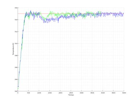
Fig. 8: Experimental results comparing recovery time with and without fault compensation schema. With fault compensation represented by green curve. Without compensation represented by blue curve.
6. Conclusions
Updating MPC models according to the fault magnitude did not provided the expected performance. In Noura et al. (2009) is presented an additive law using the residual signal. Using such approaches, the system ’s robustness scan be greatly improved when compared to the method presented in this work. The latter is clearly show when comparing the obtained IAE indexes. Also, it is important to notice that the computation time is lower since the ANN are not necessary for the additive compensation. The present work suggest that it is better to opt for additive compensation strategies rather than MPC model correction. Further works in this topic should aim putting this additive correction into a firm mathematical ground.

