


 Spanish (pdf)
 Article in xml format
 Article references
 Send this article by e-mail
 Cited by SciELO
  Similars in
SciELO
Similars in
SciELO 
 Permalink
(1. INTRODUCTION
When predictors of a regression model are correlated, multicollinearity appears. This may be a problem depending on the degree of correlation in the dataset which may be stated using the determinant of the predictors. If the predictors are linearly dependent, the determinant of the correlation matrix is equal to 0 (perfect multicollinearity); if the determinant is equal to 1, there is no multicollinearity (Stein, 1975).
Testing for multicollinearity has been studied from parametric approaches and rule of thumb proposals. Farrar and Glauber (1967) is a seminal work in the first case. They propose three different ways to do the test. In the first one, if the determinant of the correlation of the matrix of the predictors is almost equal to 1, then there is no multicollinearity. It relies on having observations that come from an orthogonal, multivariate-normal distribution. This excludes the case when dummy variables are included. The second test they propose starts by computing the principal minors of the correlation matrix of the predictors. Each minor is divided by the determinant of the correlation of the matrix, this quotient has an F-distribution if the underlying distributions are normal. In the third case, they use the partial correlation coefficients, rij of the determinant of the correlation of the matrix of the predictors. rij are compared to their off-diagonal elements and use a t-test to make a comparison. The first and second proposals in Farrar and Glauber (1967) share the fact that the underlying distributions are normal or multivariate-normal. This may be a limitation in real life applications where dummy variables, skewness and asymmetry are present in data. Then, a nonparametric approach can be useful to overcome this issue.
Some authors claim that the problem of multicollinearity should not be an issue (Leamer, 1983; Achen, 1982). They emphasize that even in the presence of multicollinearity, estimators keep being best linear unbiased estimator (BLUE) which is actually the case. So they say that the real problem is a matter of sample size. They claim that if the sample size is large enough, then multicollinearity would not be a problem. Sample size is sometimes restricted to the field of study. In economics, for example, time series of some indicators are not long enough and statistical modeling may be challenging. Nonetheless, this is changing with the availability of open source projects to access to economic data such as the World Development Indicators (The World Bank, 2021). Around the time authors like Leamer (1983) and Achen (1982) stated their concerns, the scientific community lacked of more data or computing power, so their claim needed careful attention. But things have change in regards to computing power and data. With the emerging of the Big Data era, sample size is becoming less of an issue, but the problem of multicollinearity remains (Dinov, 2016). The problem is that the presence of multicollinearity makes the estimated variances and covariances inflated. In this context, wider confidence intervals are obtained which makes it easier not to reject the null hypothesis of the coefficients in the predictors. It follows that there may be one or more coefficients with no statistical significance but with a high coefficient of determination (Gujarati et al., 2012).
Jaya et al. (2020) make a comparison of different machine learning techniques in regression such as Ridge and Lasso to obtain the technique that avoids multicollinearity. In order to detect multicollinearity however, they use Variance Inflation Factors (VIF), which can be seen as a rule of thumb approach.
In R there are several packages that try to detect multicollinearity: Imdadullah et al. (2016) and Salmerón-Gómez et al. (2021b) are two of the most recent ones. Salmerón-Gómez et al. (2021b) propose a detection method based on a perturbation of the observations but they do not perturb dummy variables. Imdadullah et al. (2016) make a review of these methods and create an R package to make overall (determinant, R-squared, among others) and individual (Klein’s rule, VIF, among others) multicollinearity diagnosis. Klein’s rule and VIF can be derived from a global and auxiliary coefficients of determination of a regressions model and a rule of thumb is applied. In this sense, both methods consider the coefficients of determination fixed when it can actually be considered a random variable (Carrodus and Giles, 1992; Koerts and Abrahamse, 1969). If by bootstrapping we let the global and auxiliary coefficients of determination be random variables, the detection of multicollinearity goes one step further. This work takes the two of the most widely used individual rule of thumb methods, Klein’s rule and VIF, and places them in a bootstrap context in order to have a statistical test to assess multicollinearity. This proposal makes it possible to have a null hypothesis and an alternative hypothesis for the presence of multicollinearity, and depending on the significance level, the researcher could reach a conclusion.
This paper is organized as follows. In Section 2, we detail the VIF, Klein’s rule, their relationship and recall the bootstrap concept. Section 3 states the null and alternative hypothesis of the proposed MTest with it corresponding procedure. In Section 4, we set up a simulation study to analyze MTest under a controlled situation. In Section 5, we apply MTest to a widely used dataset known to have multicollinearity issues. Finally, in Section 6 we give some conclusions.
2. NOTATION AND CONCEPTS
2.1 General Setup
Consider the regression model
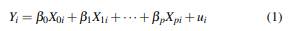
where i = 1,...,n, Xj,i are the predictors with j = 1,..., p, X 0 = 1 for all i and u i is the gaussian error term. In order to describe Klein’s rule and VIF methods, we need to define auxiliary regressions associated to model (1). An example of an auxiliary regressions is:
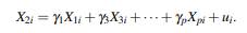
In general, there are p auxiliary regressions and the dependent variable is omitted in each auxiliary regression. Let R g 2 be the coefficient of determination of (1) and 𝑅 𝑗 2 the jth coefficient of determination of the jth auxiliary regression.
2.2 VIF
A common way practitioners compute the VIF method is by:
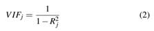
for every auxiliary regression j = 1,..., p. It states that multicollinearity is generated by covariate X j if VIF j > 10 (Gujarati et al., 2012). The case j = 0 is not considered since (2) detects approximate multicollinearity of the essential type. This means that the intercept is excluded. For more details and methods on detecting essential and non-essential multicollinearity, see Salmerón-Gómez et al. (2020).
2.3 Klein’s rule
Klein’s rule compares the 𝑅 𝑗 2 coefficient of determination of the jth auxiliary regression with 𝑅 𝑔 2 . The rule states that if 𝑅 𝑗 2 > 𝑅 𝑔 2 then the Xj variable originates multicollinearity. Klein stated that Intercorrelation ... is not necessarily a problem unless it is high relative to the over-all degree of multiple correlation . . . (Klein, 1962). It means that there is an implicit threshold ( 𝑅 𝑔 2 ) and Klein’s rule should be used along with VIF as they may be complementary since there will be cases when VIF report a multicollinearity problem, but Klein’s rule does not.
2.4 Relationship between the VIF and Klein’s rule
It is possible to link both methods by the expression
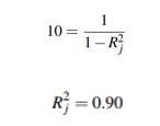
which means that according to the VIF method, variable Xj originates multicollinearity if 𝑅 𝑗 2 ≥ 0.90. Different contradictions that may exist between the Klein’s rule and the VIF. For example, if 𝑅 𝑔 2 = 0.85 and some 𝑅 𝑗 2 = 0.88, Klein’s method would detect multicollinearity but VIF will not. As another example, if 𝑅 𝑗 2 = 0.94 and 𝑅 𝑔 2 = 0.98, VIF will detect multicollinearity but Klein will not. It should be noted that the value 0.90 is not fixed in all applications. For example, works like Marcoulides and Raykov (2019) tests several values as a VIF threshold. Our proposal, MTest has 0.90 threshold by default but can be changed if the researcher decides another one.
2.5 Bootstrap
The bootstrap resampling technique was introduced by Efron, (1992), in his seminal work Bootstrap methods: Another look at the jackknife. It is a computationally intensive method, without strict structural assumptions in the underlying random process that generates the data. It is used to obtain approximations of the distribution of an estimator, of the bias, the variance, standard error and confidence intervals. In a normal experiment, repeating the experiment enables us to compute standard errors, the bootstrap principle lets us simulate the replication by resampling. If the resampling mechanism is chosen appropriately, then the resampling, together with the sample in question, is expected to reflect the original relationship between the population and the sample. The advantage is that we can now avoid the problem of having to deal with the population, and instead we can use the sample and resamples, to address statistical inference questions regarding the unknown quantities in the population. The bootstrap principle addresses the problem of not having complete knowledge of the population, to make an inference about the estimator  , schematically:
The first step consists of the construction of an estimator of an unknown probability distribution  from the available observations X
1
,...,X
n
, which provides a representative image of the population
from the available observations X
1
,...,X
n
, which provides a representative image of the population
The next step consists of the generation of random variables  of the estimator
  , which fulfills the role of the sample for the bootstrap version of the original problem.
Therefore, the bootstrap version of the estimator  based on the original sample X
1
,...,X
n
is given by
based on the original sample X
1
,...,X
n
is given by  , obtained by substituting
  .
.
The above setup is known as the nonparametric bootstrap, but it also has a parametric approach where one can assume F belonging to a parametric model {Fθ : θ ∈ Θ} where Θ is the parameter space. In this case,  where is an estimator of θ. For more details on parametric and nonparametric bootstrap, see Godfrey (2009).
It must be noted that the bootstrap also has some drawbacks. Horowitz (2001) highlights two important problems. The first one is instrumental variables estimation with ill correlated instruments and predictors. In this case, bootstrap approximations fail to be useful. The second problem is when the variance of the bootstrap estimator is high. This work does not fit in either of these cases since it is not related to instrumental variables and the variance of the bootstrap estimator is finite and well behaved.
3. MTEST
Given a regression model, Mtest is based on computing estimates of 𝑅 𝑔 2 and 𝑅 𝑗 2 from nboot bootstrap samples obtained from the dataset, 𝑅 𝑔𝑏𝑜𝑜𝑡 2 and 𝑅 𝑗𝑏𝑜𝑜𝑡 2 respectively. Therefore, in the context of MTest, the VIF rule translates into:
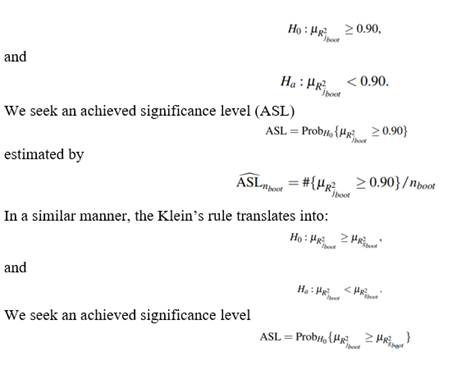
It should be noted that this set up lets us formulate VIF and Klein’s rules in terms of statistical hypothesis testing.
3.1 MTest: the algorithm
Create n boot samples from original data with replacement of a given size (nsam).
Compute 𝑅 𝑔𝑏𝑜𝑜𝑡 2 and 𝑅 𝑗𝑏𝑜𝑜𝑡 2 from each nboot samples. This outputs a B nboot ×(p+1) matrix.
Compute ASL nboot for the VIF and Klein’s rule.
Note that the matrix Bn boot ×(p+1) allows us to inspect results in detail and make further tests such as boxplots, pariwise Kolmogorov-Smirnov (KS) of the predictors and so on.
4. NUMERICAL EXPERIMENTS
4.1 Experiment 1
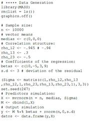
4.1.1 Data simulation
In this section, we implement the procedure described in Section 3.1 that allows us to test the hypothesis. We start by simulating 1000 data points according to the following regression:
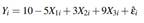
where εˆ ∼ N(0,3). X 1 , X 3 and X 3 are simulated using MASS R package (Venables and Ripley, 2002) with the following correlation structure:
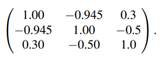
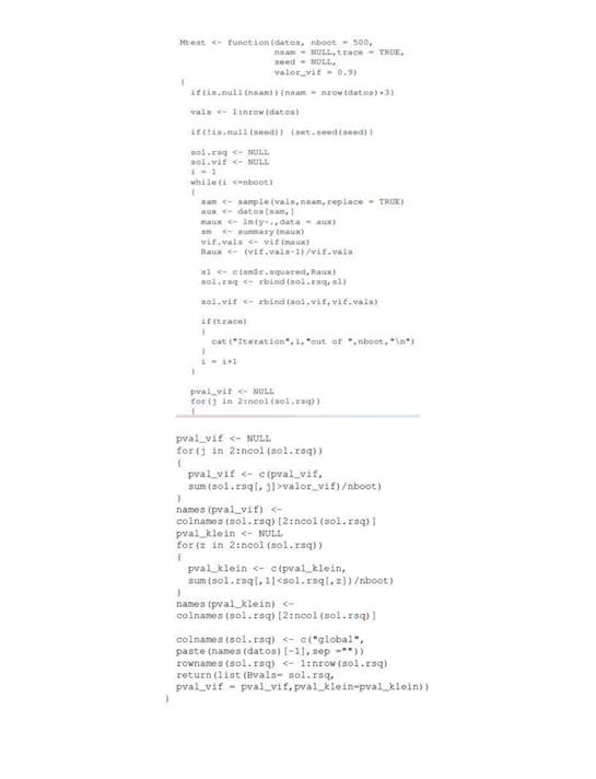
From this correlation structure it is expected that X1i and X2i may cause multicollinearity due to the high correlation between them (−0.945). The code for the data generation process is detailed in Appendix A. The code for MTest is detailed in Appendix B. The function is defined with four parameters:
• datos: A p + 2 dimensional data frame that includes the dependent variable.
• nboot: Number of bootstrap replicates. This is the n boot parameter described in Section 3.1, the default nboot = 500.
• nsam: Sample size in the bootstrap procedure. When nsam = NULL (default), then nsam = nrow(datos)*3.
• trace: Logical. If TRUE then the iteration number out of a total of nboot is printed. The default value is FALSE.
• seed: A numeric value that sets the seed value of the procedure. The default value is NULL.
• valor_vif: A numeric value that sets threshold for in the VIF rule. The default value is valor_vif=0.9
4.1.2 Testing multicollinearity
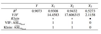
Table 1 shows the R2 for the global regression and auxiliary regressions in the first row, VIF values are presented in the second row and Klein’s rule can be computed with this information which is shown in the third row. The fourth and fifth row of Table 1 present the MTest results by computing  for VIF and Klein’s rules.
From a traditional usage of the rules, the Klein’s rule suggests that X2 is a variable that causes multicollinearity since its auxiliary regression  is greater than the global 𝑅 𝑔 2 . Kleins’s rule is presented with ∗ denoting the variables that the rule identifies as a problem and with • the variables that do not.
In the VIF case, if the threshold is equal to 10, this method suggests that X1 and X2 causes multicollinearity. Both rules detect multicollinearity problems as expected. MTest is also presented in Table 1 with ASL values computed with nboot = 1000,  for VIF and Klein are 1 for predictors X
1
, X
2
and 0 for X
3
. This implies that we cannot reject the null hypothesis stated in 3.1. In other words, this means that X
1
and X
2
also yield multicollinearity problems according to MTest which confirms the results in the application of traditional VIF and Klein’s rules.
for VIF and Klein are 1 for predictors X
1
, X
2
and 0 for X
3
. This implies that we cannot reject the null hypothesis stated in 3.1. In other words, this means that X
1
and X
2
also yield multicollinearity problems according to MTest which confirms the results in the application of traditional VIF and Klein’s rules.
Table 1 R2 for the global regression and auxiliary regressions are presented in the first row. VIF values are presented in the second row and Kleins’s rule is presented with ∗ denoting the variables that the rule identifies as a problem and with • the variables that do not
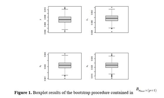
Boxplots of 𝑅 𝑔𝑏𝑜𝑜𝑡 2 and 𝑅 𝑗𝑏𝑜𝑜𝑡 2 are presented in Figure 1. They show that the bootstrap distributions are centered at their means for Y, X 1 , X 2 and X 3 , respectively are 0.9073, 0.9308, 0.9432, 0.5274. We need to leave all variables in the initial model, the MTest function also gives us a clear idea of the variability in global 𝑅 𝑔 2 : in our simulation, 0.9041 ≤ 𝑅 𝑔 2 ≤ 0.9106. This bootstrap replicates open the possibility of applying other testing methods to check how statistically different the values are. For example, we apply a Kolmogorov-Smirnov (KS) test.
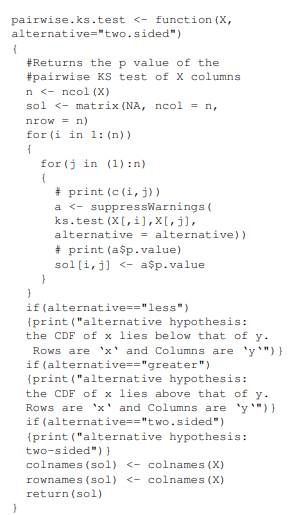
A pairwise KS matrix of p-values is presented in Tables 2 and 3, we set the significance level α = 0.05. The code for computing the pairwise KS matrix is detailed in Appendix C. Table 2 shows the pairwise p-values for the equality hypothesis of the n boot replicates of variables in the rows compared to the variables in the columns. For example, the pairwise p-value between X 2 and X 3 (0) is lower than α which rejects the equality hypothesis between them. Note that all the off-diagonal p-values also reject the hull hypothesis.

Table 3 shows the pairwise p-values of  . The null hypothesis is that the Cumulative Distribution Function of the variable in the row does lie below that of the variable in the column. In other words, we are testing if R2 values in the rows are greater than the ones in the columns. Note that the first column is similar to testing
  . For example, the first column tells us that X1 and X2 are greater than Y which is consistent with our previous findings.

Once candidate variables that may be causing multicollinearity are identified, some researchers decide to remove one or more of them. Note that results in Table 3 can also guide our decision on choosing whether X1 or X2 should be removed from the regression. If we take the sum over the rows in Table 3, this value gives us a metric that could be used to prioritize the removal of the variables. This is a metric of how much the variable in the row is greater than the one in the column. In this example, the row sum for X2 is 4 and for X1 is 3. It then suggests that X2 is the one that should be removed.
4.2 Experiment 2
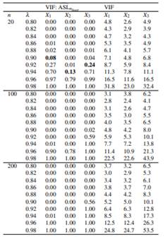
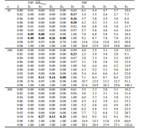
This experiment studies MTest vs rule of thumb VIF in (2) and contrasts its results. Following Salmerón-Gómez et al. (2018) and Salmerón-Gómez et al. (2021a), data is simulated as:
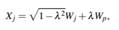
where j = 2,..., p with p = 3,4,5, Wj ∼ N(10,100), λ ∈ {0.8,0.82,0.84,...,0.98} and n ∈ {20,100,200}. This setup let us specify different grades of collinearity (λ), different sample sizes (n) and different number of covariates (p).
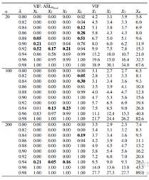
Table 4 shows results for p = 4 and Appendix D for p = 3 (Table 9) and p = 4 (Table 10). We can see that all VIF troubling values are also detected by MTest, but there are cases where MTest detects multicollinearity and VIF does not (VIF threshold is 10). For example, with α = 0.05, if λ = 0.94 and n = 100, MTest detects X2 as a variable with potential multicollinearity but VIF does not (VIF = 8.5). All such these cases are in bold.
5. APPLICATION
This section applies the proposed method to a dataset available in Longley (1967) and is used to show problems of multicollinearity. It is a time series from 1947 to 1962 where
• y: number of people employed, in thousands.
• x1: GNP implicit price deflactor.
• x2: GNP, millions of dollars.
• x3: number of people unemployed in thousands.
• x4: number of people in the armed forces.
• x5: non institutionalized population over 14 years of age. • time: year.
The regression model is given by

its global 𝑅 𝑔 2 = 0.996 and its estimation is: Table 5 shows the estimation of coefficients in equation (1). The p-value of the F statistic is closely equal to 0 which means that we can reject the null hypothesis that φ1,φ2,...,φp = 0. As mentioned in Gujarati et al. (2012), one symptom of the presence of multicollinearity is when we have a high R2 and a few significant individual predictors. Which is the case in this application since out the six predictors, only three are statistically significant.
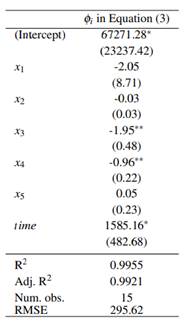
Figure 2 shows the bootstrap replicates of the dependent variable (global) and the predictors (x1 to time). Boxplots suggest that x2, x5 and time are candidate variables that generate multicollinearity problems. Furthermore, x1, x3 and x4 seem not to be greater than the dependent variable.
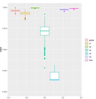
Table 6 shows the results in a similar manner that the one shown in 1. According to the traditional VIF rule, all the variables yield multicollinearity problems except in x4 (VIF threshold equal to 10). Traditional Klein’s rule shows a multicollinearity problem in predictors x2, x5 and time.
The MTest given by VIF:  shows multicollinearity problems in the same predictors that the traditional VIF did, but the value 0.003 gives us a confidence metric to reject the null hypothesis
  .
.
Setting α = 0.05, the MTest given by Klein’s: shows multicollinearity problems in predictors x1,x2, x5 and time. That is, x1 was identified as a predictor with potential multicollinearity problems but the traditional Klein did not. Note also that setting α = 0.10, we could reject the null hypothesis  ≥
≥  .
.
Table 6 R2 for the global regression and auxiliary regressions are presented in the first row. VIF values are presented in the second row and Kleins’s rule is presented with ∗ denoting the variables that the rule identifies as a problem and with • the variables that do not

Table 7 shows the pairwise p-values of  from the application data. The null hypothesis is that the Cumulative Distribution Function of the variable in the row does lie below of the variable in the column. The first column is similar to testing
 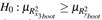 . It tells us that the predictors that are greater than the response variable are x
2
, x
5
and x
6
, which is consistent with our intuition derived from Figure 2.
. It tells us that the predictors that are greater than the response variable are x
2
, x
5
and x
6
, which is consistent with our intuition derived from Figure 2.
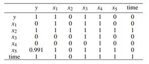
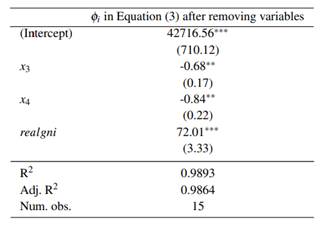
Table 7 can also help us decide which variable should be removed first. For example, in this case x 2 , time and x5 would be the order of removing the predictors. This is achieved by checking the rows of Table 7, this may suggest the ordering of the removal. Respectively, the row sums of x 2 , time and x 5 are 7, 6, and 4.991. In our application, after removing x2 from the dataset, the p-values of the Klein’s rule using MTest are 0.002, 0.000, 0.000, 0.314 and 0.845 for x 1 , x 3 , x 4 , x 5 and time respectively. Only after removing x2, time and x5 multicollinearity was removed. Nonetheless, this removal recommendation is a purely empirical approach. In this application, we could have divided x 2 by x 1 since this ratio (realgni) is a useful predictor as well, it is the real GNP. By doing this, and removing predictors x 5 and time, multicollinearity was also removed. This means that the theory behind the predictors could play a very important role when dealing with multicollinearity. The final model after this last consideration is shown in Table 8.
6. CONCLUSIONS
MTest is a bootstrap application for testing multicollinearity problems in the predictors. It lets us have a confidence metric, ASL, that given an α threshold helps us decide whether or not reject the null hypothesis stated in 3. The whole code generated for this article can be found at https://github.com/vmoprojs/ ArticleCodes/tree/master/MTest.
The application shows consistency with the numerical experiments. Both present MTest as a useful approach to test multicollinearity giving a boosting to the traditional rules in the sense that we can now have distributions of  and
and  which are involved in the testing procedure.
A graphical representation of the bootstrap replicates were found to be very useful. In our application, MTest lets us have boxplots of the predictors and the dependent variable to guide our intuition and later perform a KS test. The pairwise KS matrix of p-values is a complementary tool for testing multicollinearity derived from MTest. It can also help us decide which predictor has more potential multicollinearity problems.
This work can be extended to generalized linear models in the same manner that Fox and Weisberg (2019) did with the vif function contained in car package, but the general idea of MTest would remain the same. Another extension of MTest could be possible in the context of Ridge, Lasso or Elastic Net regression. The hyperparameters in these methods are usually selected through cross validation or repeated cross validation, and MTest could be implemented in these procedures.