SciELO - Scientific Electronic Library Online

 
vol.42 número2Riesgo de Sodicidad en los Suelos de Cantón Milagro, Guayas-Ecuador en Época de EstiajeEvaluación de productos IMERG V03 y TMPA V7 en la detección de crecidas caso de estudio cuenca del río Cañar índice de autoresíndice de assuntospesquisa de artigos
Home Pagelista alfabética de periódicos  

Serviços Personalizados

Journal

Artigo

Indicadores

Links relacionados

  • Não possue artigos similaresSimilares em SciELO

Compartilhar


Revista Politécnica

versão On-line ISSN 2477-8990versão impressa ISSN 1390-0129

Rev Politéc. (Quito) vol.42 no.2 Quito Nov./Jan. 2019


Articles

Algebraic IDA-PBC for Polynomial Systems with Input Saturation: An SOS-based Approach

IDA-PBC Algebraico Para Sistemas Polinomiales con Saturación en las Entradas: Un Enfoque Basado en SOS

Oscar B. Cieza A. 1   *  

Johann Reger 1  

1Technische Universität Ilmenau, Grupo de Ingeniería de Control, Ilmenau, Alemania


Abstract:

The necessity to deal with partial differential equations (PDEs) and the dissipation condition are the main adversities in the application of Interconnection and Damping Assignment Passivity-Based Control (IDA-PBC). Recently, an algebraic solution of IDA-PBC has been explored for a class of affine polynomial systems by using sum of squares (SOS) and semidefinite programming (SDP). In this work, we extend the previous method by incorporating actuator saturation (AS) and two minimization objectives in the SDP. Our results are validated on two polynomial systems.

Keywords: Port-Hamiltonian Systems; IDA-PBC; Polynomial Systems; Sum of Squares; Actuator Saturation

Resumen:

La solución de ecuaciones diferenciales parciales (PDE) y la condición de disipación son las principales adversidades en la aplicación de Interconnection and Damping Assignment Passivity-Based Control (IDA-PBC). Recientemente, se ha explorado una solución algebraica de IDA-PBC para una clase de sistemas polinomiales utilizando el método de suma de cuadrados (SOS) y la programación semidefinida (SDP). En este trabajo se amplía el método anterior incorporando saturación en los actuadores (AS) y dos objetivos de minimización en la SDP. Nuestros resultados son validados en dos sistemas polinómicos.

Palabras clave: Sistemas Port-Hamiltonianos; IDA-PBC; Sistemas Polinomiales; Suma de Cuadrados; Saturación del Actuador

1. INTRODUCTION

Over the last decade, Interconnection and Damping Assignment Passivity-Based Control (IDA-PBC) has experienced increasing practice due its wide applicability (Petrovi´c et al., 2001; Batlle et al., 2004, 2007; Ortega and García-Canseco, 2004; Li et al., 2010; Astolfi and Ortega, 2001; Fujimoto et al., 2001; Renton et al., 2012; Li et al., 2013; Astolfi et al., 2002a; Xue and Zhiyong, 2017). The standard IDA-PBC method requires a two step procedure: energy shaping and damping injection. The first depends on the solution of partial differential equations (PDEs) and the second together with zero state detectability (ZSD) of the closed-loop guarantees asymptotic stability.

In order to simplify the PDE problem Viola et al. (2007) have introduced a change of coordinates and a modification of the target dynamics. With the objective to completely avoid PDEs, the following leading methods have been proposed: constructive procedures (Donaire et al., 2016a; Borja et al., 2016; Romero et al., 2017), implicit port-Hamiltonian representation (Macchelli, 2014; Castaños and Gromov, 2016) and an algebraic approach (Fujimoto and Sugie, 2001; Batlle et al., 2007; Nunna et al., 2015). In addition, it has been shown in (Batlle et al., 2007; Donaire et al., 2016b) that a two step IDA-PBC may be restrictive in some cases, thus introducing a single step procedure (SIDAPBC). Furthermore, dissipation in the under-actuated degrees of freedom, see (Gómez-Estern and Van der Schaft, 2004), may also turn out an obstacle for the implementation of IDA-PBC on some systems, e.g. on the cart-pole system (Delgado and Kotyczka, 2014).

It is well-known that actuator saturation (AS) can cause performance losses or even lead to closed-loop instability. In this context, Åström et al. (2008); Escobar et al. (1999) have studied PBC with AS on two specific systems. Sun et al. (2009); Wei and Yuzhen (2010) analyze stability for saturation in the damping injection term. A variable structure approach to energy shaping for a class of Port-Hamiltonians system is developed in (Macchelli, 2002; Macchelli et al., 2003). Besides, Sprangers et al. (2015) studied a reinforcement learning method for energy shaping which shows robust properties under AS.

In polynomial systems the sum of squares (SOS) approach with semidefinite programming (SDP) allows to synthesize Lyapunov functions (Parrilo, 2000), optimal (Ichihara, 2009), robust (Zhu et al., 2018; Jennawasin et al., 2010), fuzzy (Wibowo et al., 2014; Yu and Wang, 2013) and AS-focused controllers (Jennawasin et al., 2012; Valmorbida et al., 2013; Ichihara, 2013), among others. This AS controllers, calculated with SOS, use the polytope representation introduced in (Hu and Lin, 2001) for linear system with multiple input saturation.

For a class of polynomial affine systems, lately, Cieza and Reger (2018) have presented an algebraic method the conditions of which are met by means of SOS and SDP solutions. The method solves the typical problems of IDA-PBC at the expense of an adequate parametrization and selection of the Hamiltonian. To the best knowledge of the authors there is no definitive solution to the AS controller design problem with IDA-PBC. The underlying work shall now also incorporate AS and two minimization objectives in the SDP solver, extending the algorithm of Cieza and Reger (2018).

The work is organized as follows. We summarize the concepts of IDA-PBC for nonlinear affine systems in Section 2. Section 3 recapitulates the algebraic method of Cieza and Reger (2018). In Section 4 we solve the AS problem in the algebraic approach using additionally two minimization objectives. We discuss the application of SOS methodology and verify our results in Section 5, applying the approach on two polynomial systems. Finally, we draw our conclusions in Section 6.

2. IDA-PBC FOR AFFINE NONLINEAR SYSTEMS

Let us recall the IDA-PBC approach for nonlinear affine systems introduced by Ortega and García-Canseco (2004). Consider the system

x˙=f(x)+g(x)u (1)

and the target port-Hamiltonian system

x˙=Fd(x)Hdx(x), (2)

where XhRnx is the state space manifold,  Rm is the input space, g has full rank, the skew symmetric portion 12(Fd-Fd)Rnx×nx is the interconnection matrix, the symmetric portion Rnx×nx12(Fd+Fd)0 is the dissipation matrix and Hd:XhR with x=argminHd(x) is the desired positive definite Hamiltonian. If the matching condition (If in the matching condition (3) the structure of Fd(x) is fixed, then (3) is a PDE. If H(x) is fixed, then (3) is an algebraic equation.)

g(x)f(x)=g(x)Fd(x)Hdx(x) (3)

is fulfilled for some Fd,Hd and full rank left annihilator (The full rank left annihilator g is given by g(x)g(x)=0 and rank(g)=nx-m. Consequently, (3) exists iff nx>m.) g then the control law

uI=g(x)g(x)-1g(x)Fd(x)Hdx(x)-f(x)

transforms (1) into the stable system (2) with Lyapunov function Hd. Asymptotic stability of x in the attainable set Xa={xXhgf=0} may be demonstrated e.g. by using passivity with Lyapunov stability theory, see (Astolfi et al., 2002b; Sepulchre et al., 1997).

3. IDA-PBC FOR POLYNOMIAL SYSTEMS

In this section we summarize Proposition 4–5 from (Cieza and Reger, 2018) for β = 1. The variable β of the aforementioned work can be considered as a scaling factor, which does not alter our main results.

3.1 Algebraic IDA-PBC

Let Γ(x),g(x),g(x), and g(x)f(x) be polynomial functions in

Γ(x)x˙=f(x)+g(x)u (4)

and the desired closed loop port-Hamiltonian system

Γ(x)x˙=g(x)g(x)-1F(x)Hdx(x), (5)

where

F(x)=F1(x)F2(x),  Hd(x)=z(x)P-1z(x),  P=P0

Without loss of generality let argminHd(x)=0. Besides, state and input spaces remain as in (1), z:XhRnz is a vector of polynomials with nznx, PRnz×nz is a constant matrix, F,Γ:XhRnx×nx are full rank polynomial matrices (Invertibility of Γ enables (4) to take the usual form x˙=f¯(x)+g¯(x)u and Fd(x)=Γ-1(x)g(x)g(x)-1F(x)), and F holds the portions F2xRm×nx and F1(x)Rnx-m×nx.

Proposition 1 Closing the loop of system (4) with control

ub=(gg)-1 F2zxP-1z-gf (6)

renders the equilibrium point x=0 of the closed loop system (5) locally stable for any initial state x(0)=x0XP={xRnxHd(x)=z(x)P-1z(x)1} whenever the following conditions are fulfilled for all xXh=xRnx0h(x)=1-z(x)Sh-1z(x),Sh0.

C1 There exist polynomial functions Λ1x, gx and z(x) such that gxfx=Λ1xzx and zx=0 iff x=0. Besides, if nz=nx then zx is unimodular (Polynomial matrices are unimodular if the inverse matrix again is a polynomial matrix. Their determinant always is a non-zero constant), else zx has rank nx and zxxPΛ1x=0 whit zx he full rank left annihilator of the Jacobian of z.

C2 There is a polynomial function Nx such that if nz=nx then Nx=zx-x, else zxxNx=Inx and N zx is a full rank square matrix. (Here In represents the identity matrix of size n.)

C3 There is a constant matrix P, and polynomial matrices 0S1(x)Rnx×nx and F2(x) such that

-Φ(x)-Φ(x)-h(x)S1(x)0 (7)

ShPz(x0)z(x0) (8)

Φ=ggΓF1F2,  F1(x)=Λ1(x)PN(x)

Furthermore, the origin of (5) is asymptotically stable if

-Φ(x)-Φ(x)-h(x)S1(x)0 (9)

for nz>nx,  zxxP-1zx=0 implies x=0

Proof 1 It can be found in (Cieza and Reger, 2018) with a modification of (8) using the Schur complement.

3.2 Existence of ub

The next proposition provides a sufficient condition for the existence of F2, i.e. the existence of the (asymptotically) stabilizing control law (6).

Proposition 2 Consider x0XPXh and asume Λ1, g, z, N are selected according to C1 and C2. Then there exists a function F2x that meets C3 if there exists P=P0 and S2x0 such that

-ϕx-ϕx-hxS2x0, ϕx=gxΓxF1x=gxΓxNxPΛ1x, (10)

with ϕx, S2xRnx-m×nx-m. Additionally, (9) is solvable as long as

-ϕ(x)-ϕ(x)-h(x)S2(x)0 (11)

Lastly, if (10) or (11) are satisfied, then a solution for F2 with 0Lx+LxRm×m is

F2=-g(x)Γ(x)F1(x),L(x)g(x)g(x)-Γ-(x) (12)

Proof 2 See (Cieza and Reger, 2018, Prop. 5).

Application of the algorithm starts with adequate selection of Λ1, z, g and N according to (4), (5), C1 and C2. Later, we choose h and solve (for convenience) (7), (9), (10) or (11) searching for P (and F2 in case of Prop. 1) under (8) which defines an upper and lower bound on P, namely x0XPXh for some given x0.

In comparison, Proposition 2 requires the solution of smaller LMIs to calculate the parametrized function F2, see (12), or to guarantee its existence, whereas Prop. 1 defines F2 as general function s.t. (7) (and (9)) is satisfied, which grants more flexibility at the expense of computational cost. In order to use SOS with SDP we force F2 (in Prop. 1) to be a polynomial function of some selected degree.

Proposition 2 can also be used as a fast indicator such that Proposition 1 will work. Note that Proposition 2 contains the minimal conditions that P, Λ1, g, N, h and Γ have to satisfy, and it guarantees the existence of a not necessarily polynomial function F2. Hence, if we constrain F2 to be polynomial, then Proposition 2 is experimentally still a good, but not an unconditionally reliable reference.

4. MAIN RESULTL

In view of Proposition 1 and 2, we extend the results of Cieza and Reger (2018) to consider actuator saturation (AS). In addition, we define two possible minimizations (optimization objectives) for the SDP.

4.1 Actuator Saturation (AS)

Proposition 3 Let all conditions of Prop. 1 for local (asymptotic) stability be satisfied and assume:

C5 There exist polynomial matrices Λ2(x)Rm×nz and 0S3(x)Rm×m such that

Λ1(x)Λ2(x)z(x)=g(x)g(x)f(x) (13)

η11(x)η12(x)η12(x)P0, η11x=ggx Suxggx-hxS3x, η12x=F2xzxx-Λ2xP. (14)

Then the stabilizing control law (6) is restricted to Ub=ubUubSu-1xub1 with Rm×mSux=Sux0x for anyXP.

Proof 3 Multiplying (14) on both sides by adequate matrices and using the Schur complement yields

Im-WWhSu-12(gg)-1S3(gg)-1Su-12 (15)

with W(x)=Su-12(gg)-1F2zxP-12-Λ2P12and P12P12=P. Now taking the spectral norm on 15for xXPXh, i.e. h0, and the definition of XP as P-12z221 we have

1Su-12(gg)-1F2zxP-12-Λ2P1222

Su-12(gg)-1F2zxP-12-Λ2P1222P-12z22

Su-12(gg)-1F2zxP-1z-Λ2z22

=Su-12ub22=ubSu-1ub

where last equalities are obtained with (13) and (6).

After solving the conditions of Proposition 1 and 3, we may calculate a control input ubUb, for any xXP. Proposition 3 can also be extended to work with Prop. 2 by replacing (12) in (14). This yields an LMI which is not necessarily polynomial. Therefore, we restrict L to be polynomial and multiply (14) on the right with the square non-singular matrix. (Note that using C2, the square matrix Nzx and as a consequence NΓg,NΓg,zx has full rank.)

Im0000N(x)Γ(x)g(x)N(x)Γ(x)g(x)zx(x)

and on the left by its transpose. This results in conditions that can be solved by means of SOS + SDP

Following the works of Hu and Lin (2001); Valmorbida et al. (2013); Ichihara (2013), among others, we may use the polytope or polytopic saturation model within the algebraic IDA-PBC, as phrased in the following proposition.

Proposition 4 Let the conditions of Propositions 1 and 3 be satisfied for some system of the form (4) resulting in some matrices P, F2 and a locally (asymptotically) stabilizing constrained controller u=ubUb given by (6). Consequently, there is a new (asymptotically) stabilizing control action

usUs=us=ub+(gg)-1Θuδ|θk[0,1], uδ=(F21-F20)(diffzx)P-1z,     F2=F20 (16)

provided that there exist matrices F21xRm×nz and S¯i1imx0,s.t. for all ik0,1 with k=1m,

-Φi1imx-Φi1imx-hxS¯i1imx0,  Φi1im=ggΓF1F2i1(x)e1F2im(x)em (17)

where Θ=diagθ1,,θm and ei the ith unity vector. In addition, asymptotic stability is achieved if (9) are satisfied and (17) is strict.

Proof 4 Define

F2=ΘF21+(Im-Θ)F20,(polytope) (18)

and βk0+βk1=1, θk=βk0, then (16) follows from (6) and (18). Then, replace (18) in (7), multiply it by ik=01βkik for convenience and substitute S1 with S¯i1im which does not affect stability, see (Cieza and Reger, 2018). Then (7) results in

0i1=01β1i1im=01βmim(-Φi1im-Φi1im-hS¯i1im)

and rewritten as a sum of positive semidefinite polynomial functions (convex set) this yields

0j=02m-1β¯j(-Φj-Φj-hS¯j) (19)

with j=k=1mik2k-1, j=02m-1β¯j=1. Therefore, a sufficient condition for (19) is (17). The proof of asymptotic stability follows a similar procedure.

Proposition 4 implies that if there is a solution to the conditions of Propositions 1 and 3 with (17), then there also exists an (asymptotically) stabilizing control law (16). In addition, if F2=F20=F21 then (16) is reduced to (6) and (17) becomes (7) (or (10)). Proposition 4 can be easily extended to work with Prop. 2 (instead of 1). In this case, (17) is reduced to

Li1e1Limem+Li1e1Limem0,  F2i=-gxΓxF1x,Lixgg-Γ-x.

In the same way as in (Hu and Lin, 2001; Valmorbida et al., 2013; Ichihara, 2013) for multiple input systems, we can adopt the independent input saturation given by usat-i=satux,u¯,u_ and ux=ub+gguδ, where u¯ and u_ are maximum and minimum values of ub in Ub. Figure 1 illustrates the situation for m=2, gg=I2, ux, ub, usat-i and sets Ub, Us.

Figura 1.  Relations of u constrained and saturated. 

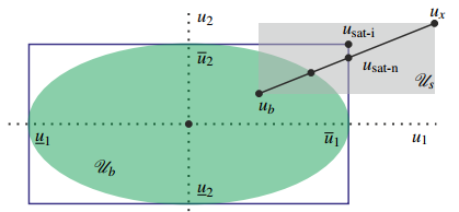
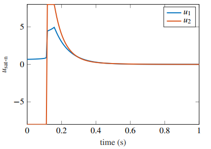
Here, we also observed that in order to have AS, independent input saturation (usat-i) is not the only solution. Therefore, to simplify (17), we select θ1=θ2==θm and a new saturation function given by

usat-n=ub+(gg)-1uδ minρ1,,ρm,  Pk=ek(u¯-ub)ek(gg)uδ,ifekux>eku¯,ek(gg)uδ0,ek(u_-ub)ek(gg)uδ,ifekux<eku_,ek(gg)uδ0,1,otherwise,

which is also shown in Figure 1. Selection of usat-n reduce 2m-1 inequalities and polynomial matrices S¯ in (17).

4.2 Optimization Objectives in SDP

Proposition 1–3 only guarantee a solution for P and F2(x) without any performance or optimization goal in the SDP. In addition, we may set the following simple objectives:

Optimization 1 (Volume maximization of XP)

minimize     traceY, subject to     PInzInzY 0 (20)

Proof 5 The volume of XP is proportional to det(P), see (Boyd et al., 1994, pp. 48-49). In addition, from KL-divergence between two multivariate normal distributions, we obtain the relation

trace(Inz-A-1)log(det(A))trace(A-Inz) (21)

for any real matrix A0. Therefore, maximizing the volume of XP with P0 is equivalent to maximize logdetP. Using (21) we enlarge the minimum bound of log(det(P)) by minimization of trace(P-1) which is equivalent to Opt. 1 with Schur complement in (20).

This minimization is also used empirically in (Ichihara, 2013). Optimization 1 maximizes the volume of XP by maximizing the minimum bound of P given by Y-1. Note that searching for the biggest XP does not demand the explicit selection of x0 (right hand side of (8)).

Optimization 2 (Volume minimization of Ub)

minimizetrace(Su)subject toSu=constant

Proof 6 Along the same lines of Optimization 1, except that we consider the upper bound of (21).

Without loss of generality, define F2x=F¯2xPNx, 0=F¯2xPzxx, for some function F¯2Rm×nz. Then, (14) becomes

(gg)Su(gg)-(F¯2-Λ2)P(F¯2-Λ2)0

for all xXh. This shows that minimization of Su (upper bound of u) is equivalent to minimize F¯2-Λ2 and an upper bound of P. As a consequence, it is required to have at least one minimum bound on P (right hand side of (8) or Opt. 1).

5. SIMULATIONS

It is well-known that the SOS property is a sufficient condition for checking the non-negativity of a polynomial function (Parrilo, 2000). For this reason, we may search for positive semidefinite matrices that are matrix SOS polynomials in Propositions 1–4. To guarantee strict inequalities in the SDP solver, we add 10-3Inz in P0, 10-3Inx-m in (10), and 10-3In in (7 and (17). The algorithm is processed in Matlab by use of SOSTOOLS and SDPT3, see (Papachristodoulou et al., 2016). For details on the transformation from SOS to SDP see (Parrilo, 2000).)

In the following examples we search for asymptotically stabilizing controllers wrt. two systems using the results of Proposition 1–4. Values presented in this paper have been rounded to three decimals for better visibility.

5.1 Nonlinear Second Order System

We shall test Proposition 1–3 for synthesizing an asymptotically stabilizing constrained controller in the system

x˙1x˙2=x12+x2x1+01u

First, we pick z(x)=[x1,x12+x2], g=1,0, Γ=I2, Λ1=0,1, and  Λ2=1,0. Thus, zx  is unimodular and C1C2 are satisfied. Then we select Sh=diag9,9, S1xR2×2 with polynomials of degree 2 as elements and test Proposition 1 with Optimization 1 maximizing XP, obtaining XP=xR2γx1, with γ(x)=9x14-0.001x13+18x12x2+9.0x12-0.001x1x2+9x22.

Next, for illustration we select (a minimum bound on P) x0=[0,2]XP (previously found) and solve (for a new P and F2) the conditions of Prop. 1 and 3 with Opt. 2 (minimization of Su) for S3(x)R a polynomial of degree 6, resulting in Su = 100.134.

Finally, we evaluate Prop. 1 and 3 with Opt. 1 selecting, for instance, Ub=uRSu=112u2. The results can be seen in Figure 2, which shows sets XPXh, XPUb, and the phase portrait in x1-x2 plane of the closed-loop for 10 extreme initial positions x0 represented by symbol *. Here all trajectories converge to the origin as expected. In addition, Figure 3 illustrates 5 seconds of respective control actions (calculated with (6)), which are all constrained in Ub. As mentioned in Section 4, we can also use Prop. 2–3. Table 1 shows a comparison between both Propositions for x0=0,2XP, Su=112. We conclude that Prop. 2 yields better optimization results.

Figura 2.  Sets XP,Xh, Ub, and phase portrait for 10 extreme initial positions. 

Tabla 1.  Comparison of Prop. 1, 2 in Sec. 5.1. 

Prop. 1, 3 Prop. 2, 3
Opt. 1: det(P) 35.198 41.064
Opt. 2: Su 100.134 87.345

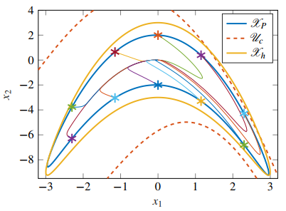
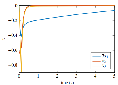
5.2 Third Order Multiple Input System with AS

Now, we consider a third order system given by
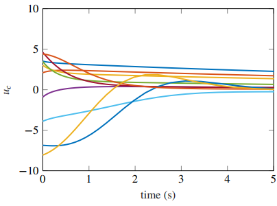
1x10-x110001x˙1x˙2x˙3=x2-2x3-2x1x2-2x22x1x2+u1x2x3+u2,

Figura 3.  Response of control signal ub (ub stays in Ub). 

with AS using usat-n, θ1=θ2. In the controller synthesis according to C1-C2, we choose g=1,0,0,

Λ1=01-2, Λ2(x)= x2000x30, Γ =1x10-x110001

and z(x)=[x1,x2,x22+x1x2+x3] unimodular zx. This example is computationally more challenging. Therefore, we select Sh=diag100,100,100 and use Prop. 2 as fast indicator that Prop. 1 will work, which is met successfully. Then, we take S1R3×3, F20x,F21xR2×3, and S3xR2×2 with polynomials of degree 2 and 4, respectively, and apply Propositions 1, 3, 4 with Opt. 1 for the user defined The minimum Sucan be found similarly as in Example 5.1. choice  Su=diag102,82.

For avoiding excessively large ux, we constrain each of the constant elements of F21 represented by fij with |fij|<10. The results are illustrated in Figures 4 and 5. Figure 4 shows the states (x1 scaled for clarity) in closed-loop under initial condition [0,-0.65,0]=x0XPXh. It is clearly seen that all states will converge to the origin. Figure 5 illustrates the first second of usat-n. Note that u2 is saturated, obviously, without compromising stability. Furthermore, using Prop. 2 in this system gives worse optimization results, which shows that the selection of the best Proposition (1 or 2) is system dependent.

Figura 4.  States with x0=[0,-0.65,0] for the third order system in closed loop. 

Figura 5.  Saturated control action usat-n

6. CONCLUSION

In this paper we provide an algebraic solution for IDA-PBC that is able to resolve the problem of actuator saturation. To this end, we restrict the design to a class of polynomial systems that yield conditions which are solvable with SOS and SDP. The presented algorithm requires the following steps:

S1 Select Λ1, Λ2,z, g and h.

S2 define Su and calculate ub with Propositions 1 or 2, 3 and Opt. 1 to maximize the volume ofXP. The minimum Su can also be calculate with Opt.2.

S3 Compute uδ with Prop. 4 and P, F2 found in S2.

S4 Implement the saturation functions usat-i or usat-n.

Additionally, we enjoy features as: no need to solve a PDE, dissipation in design, and one step IDA-PBC. Simulations of two polynomial example systems validate our approach.

ACKNOWLEDGMENT

The first author would like to acknowledge the financial support obtained from: (1) Deutscher Akademischer Austauschdienst, Germany, and (2) Programa Nacional de Becas y Crédito Educativo, Peru. The second author would like to acknowledge the financial support from European Union Horizon 2020 research and innovation program, Marie Skłodowska-Curie grant agreement No. 734832.

REFERENCIAS

Astolfi, A., Chhabra, D., and Ortega, R. (2002a). Asymptotic Stabilization of Some Equilibria of an Underactuated Underwater Vehicle. Systems & Control Letters, 45:193–206. [ Links ]

Astolfi, A. and Ortega, R. (2001). Energy-Based Stabilization of Angular Velocity of Rigid Body in Failure Configuration. Journal of Guidance, Control, and Dynamics, 25(1):184–187. [ Links ]

Astolfi, A., Ortega, R., and Sepulchre, R. (2002b). Stabilization and Disturbance Attenuation of Nonlinear Systems Using Dissipativity Theory. European Journal of Control, 8(5):408–431 [ Links ]

Åström, K. J., Aracil, J., and Gordillo, F. (2008). A family of smooth controllers for swinging up a pendulum. Automatica, 44(7):1841–1848 [ Links ]

Batlle, C., Dòria-Cerezo, A., Espinosa-Pérez, G., and Ortega, R. (2007). Simultaneous interconnection and damping assignment passivity-based control: Two practical examples. In Lagrangian and Hamiltonian Methods for Nonlinear Control 2006, pages 157–169. Springer. [ Links ]

Batlle, C., Doria-Cerezo, A., and Ortega, R. (2004). Power flow control of a doubly-fed induction machine coupled to a flywheel. In International Conference on Control Applications, volume 2, pages 1645–1650. [ Links ]

Borja, P., Cisneros, R., and Ortega, R. (2016). A constructive procedure for energy shaping of port-Hamiltonian systems. Automatica, 72(1):230–234. [ Links ]

Boyd, S., El Ghaoui, L., Feron, E., and Balakrishnan, V. (1994). Linear Matrix Inequalities in System and Control Theory, volume 15. SIAM studies in Applied Mathematics. [ Links ]

Castaños, F. and Gromov, D. (2016). Passivity-Based Control of Implicit Port-Hamiltonian Systems with Holonomic Constraints. Systems & Control Letters, 94(1):11–18. [ Links ]

Cieza, O. B. and Reger, J. (2018). IDA-PBC for Polynomial Systems : An SOS-based Approach. In IFAC Conference on Modelling, Identification and Control of Nonlinear Systems (MICNON), pages 366–371. [ Links ]

Delgado, S. and Kotyczka, P. (2014). Overcoming the Dissipation Condition in Passivity-based Control for a class of mechanical systems. In IFAC World Congress, pages 11189–11194. [ Links ]

Donaire, A., Mehra, R., Ortega, R., Satpute, S., Romero, J. G., Kazi, F., and Singh, N. M. (2016a). Shaping the Energy of Mechanical Systems Without Solving Partial Differential Equations. IEEE Transactions on Automatic Control, 61(4):1051–1056. [ Links ]

Donaire, A., Ortega, R., and Romero, J. G. (2016b). Simultaneous Interconnection and Damping Assignment Passivity-based Control of Mechanical Systems Using Generalized Forces. Systems & Control Letters, 94(1):118–126. [ Links ]

Escobar, G., Ortega, R., and Sira-Ramírez, H. (1999). Output Feedback Global Stabilization of a Nonlinear Benchmark System Using a Saturated Passivity Based Controller. IEEE Transactions on Control Systems Technology, 7(2):289–293. [ Links ]

Fujimoto, K., Sakurama, K., and Sugie, T. (2001). Trajectory tracking control of port-controlled Hamiltonian systems and its application to a magnetic levitation system. In Conference on Decision and Control, pages 3388–3393 [ Links ]

Fujimoto, K. and Sugie, T. (2001). Canonical transformation and stabilization of generalized Hamiltonian systems. Systems & Control Letters, 42(9):217–227. [ Links ]

Gómez-Estern, F. and Van der Schaft, A. (2004). Physical Damping in IDA-PBC Controlled Underactuated Mechanical Systems. European Journal of Control, 10(5):451–468. [ Links ]

Hu, T. and Lin, Z. (2001). Control Systems with Actuator Saturation: Analysis and Design. Birkhäuser. [ Links ]

Ichihara, H. (2009). Optimal Control for Polynomial Systems Using Matrix Sum of Squares Relaxations. IEEE Transactions on Automatic Control, 54(5):1048–1053. [ Links ]

Ichihara, H. (2013). A Convex Approach to State Feedback Synthesis for Polynomial Nonlinear Systems with Input Saturation. SICE Journal of Control, Measurement, and System Integration, 6(3):186–193. [ Links ]

Jennawasin, T., Kawanishi, M., Narikiyo, T., and Lin, C.-L. (2012). An Improved Stabilizing Condition for Polynomial Systems with Bounded Actuators: An SOS-Based Approach. In IEEE International Symposium on Intelligent Control (ISIC), pages 258–263. IEEE. [ Links ]

Jennawasin, T., Narikiyo, T., and Kawanishi, M. (2010). An improved SOS-based stabilization condition for uncertain polynomial systems. In SICE Annual Conference 2010, pages 3030–3034. [ Links ]

Li, H., Wang, X., and Tian, T. (2010). The performance research of induction motor systems controlled by the IDA-PBC method and its speed sensorless implementation. In International Conference on Electrical Machines and Systems (ICEMS), pages 680–683. [ Links ]

Li, J., Liu, Y., Li, C., and Chu, B. (2013). Passivity-based nonlinear excitation control of power systems with structure matrix reassignment. Information, 4(3):342–350. [ Links ]

Macchelli, A. (2002). Port Hamiltonian systems: A unified approach for modeling and control finite and infinite dimensional physical systems. Ph.d. dissertation, University of Bologna. [ Links ]

Macchelli, A. (2014). Passivity-Based Control of Implicit PortHamiltonian Systems. SIAM Journal on Control and Optimization, 52(4):2422–2448. [ Links ]

Macchelli, A., Melchiorri, C., Secchi, C., and Fantuzzi, C. (2003). A variable structure approach to energy shaping. In European Control Conference (ECC), pages 1309–1314. [ Links ]

Nunna, K., Sassano, M., and Astolfi, A. (2015). Constructive Interconnection and Damping Assignment for Port-Controlled Hamiltonian Systems. IEEE Transaction on Automatic Control, 60(9):2350–2361. [ Links ]

Ortega, R. and García-Canseco, E. (2004). Interconnection and Damping Assignment Passivity-Based Control: A Survey. European Journal of Control, 10(5):432–450. [ Links ]

Papachristodoulou, A., Anderson, J., Valmorbida, G., Prajna, S., Seiler, P., and Parrilo, P. A. (2016). SOSTOOLS: Sum of squares optimization toolbox for MATLAB. User’s guide. [ Links ]

Parrilo, P. A. (2000). Structured Semidefinite Programs and Semialgebraic Geometry Methods in Robustness and Optimization. PhD thesis, California Institute of Technology. [ Links ]

Petrovic, V., Ortega, R., and Stankovi, A. M. (2001). Interconnection and damping assignment approach to control of PM synchronous motors. IEEE Transactions on Control Systems Technology, 9(6):811–820. [ Links ]

Renton, C., Teo, Y. R., Donaire, A., and Perez, T. (2012). Active control of car suspension systems using IDA-PBC. In Australian Control Conference, pages 361–366. [ Links ]

Romero, J. G., Donaire, A., Ortega, R., and Borja, P. (2017). Global Stabilisation of Underactuated Mechanical Systems via PID Passivity-Based Control. In IFAC World Congress, pages 9577–9582. [ Links ]

Sepulchre, R., Jankovic, M., and Kokotovi, P. V. (1997). Constructive nonlinear control. Springer. [ Links ]

Sprangers, O., Lopes, G. A. D., and Babuska, R. (2015). Reinforcement learning for port-Hamiltonian systems. IEEE Transactions on Cybernetics, 45(5):1017–1027. [ Links ]

Sun, W., Lin, Z., and Wang, Y. (2009). Global Asymptotic and Finite-gain L2 Stabilization of Port-Controlled Hamiltonian Systems Subject to Actuator Saturation. In American Control Conference (ACC), pages 1894–1898. [ Links ]

Valmorbida, G., Tarbouriech, S., and Garcia, G. (2013). Design of polynomial control laws for polynomial systems subject to actuator saturation. IEEE Transactions on Automatic Control, 58(7):1758–1770. [ Links ]

Viola, G., Ortega, R., Banavar, R., Acosta, J. A., and Astolfi, A. (2007). Total Energy Shaping Control of Mechanical Systems: Simplifying the Matching Equations Via Coordinate Changes. IEEE Transactions on Automatic Control, 52(6):1093–1099. [ Links ]

Wei, A. and Yuzhen, W. (2010). Stabilization and H¥ control of nonlinear port-controlled Hamiltonian systems subject to actuator saturation. Automatica, 46(12):2008–2013. [ Links ]

Wibowo, B. S., Trilaksono, B. R., and Syaichu-Rohman, A. (2014). H¥ Control of Polynomial Fuzzy Systems: A Sum of Squares Approach. Journal of Engineering and Technological Sciences, 46(2):152–169. [ Links ]

Xue, L. and Zhiyong, G. (2017). Control of Underactuated Bridge Cranes: A Simplified IDA-PBC Approach. In 11th Asian Control Conference (ASCC), pages 717–722. [ Links ]

Yu, A. G.-R. and Wang, B. S.-M. (2013). Polynomial Fuzzy Control of an Inverted Pendulum System by Sum-of-Squares Approach. In IEEE International Symposium on Next-Generation Electronics (ISNE), pages 236–239. IEEE [ Links ]

Zhu, Y., Zhao, D., Yang, X., and Zhang, Q. (2018). Policy Iteration for H¥ Optimal Control of Polynomial Nonlinear Systems via Sum of Squares Programming. IEEE Transactions on Cybernetics, 48(2):. [ Links ]

Published: 31/01/2019

Received: October 30, 2018; Accepted: October 31, 2018

* oscar.cieza@tu-ilmenau.de

Oscar B. Cieza A. received the B.Sc. degree in Electronics Engineering in 2011 from the Pontificia Universidad Católica del Perú, Lima, and in 2014 the M.Sc. double degree in Mechatronics Engineering from the Technische Universität Ilmenau, Germany, and the Pontificia Universidad Católica del Perú. He is a doctoral student with the Control Engineering Group at TU Ilmenau since October 2015. His research interests include Interconnection and damping assignment passivitybased control (IDA-PBC) as well as robust control of underactuated mechanical systems.

Dr. Johann Reger received his diploma degree (Dipl.-Ing.) in Mechanical Engineering in 1999 and his doctorate (Dr.-Ing.) in Control Engineering in 2004, both from the University of Erlangen-Nuremberg in Germany. He has held several postdoc positions, among others, with the Mechatronics Department at CINVESTAV-IPN in Mexico-City, the EECS Control Laboratory at the University of Michigan in Ann Arbor, and the Control Systems Group at TU Berlin. Since 2008 he is a full professor and head of the Control Engineering Group at the Computer Science and Automation Faculty, TU Ilmenau, in Germany. There he also serves as vice-dean and director of the Institute for Automation and Systems Engineering. His current research foci are on adaptive and robust control, variable structure and sliding mode control, state and parameter estimation. Application areas include robotics, mechatronics, automotive, and water systems.

Creative Commons License This is an open-access article distributed under the terms of the Creative Commons Attribution License