


 Espanhol (pdf)
 Artigo em XML
 Referências do artigo
 Enviar este artigo por email
 Citado por SciELO
  Similares em
SciELO
Similares em
SciELO 
 Permalink
INTRODUCTION
Nowadays, wind energy has grown because of the high demands of renewable energies worldwide. In this context, energy efficiency must be improved in order to obtain as much energy as possible from the source [1], [2], [3]. For wind turbines, the transition from no load to full load operation is crucial for the control of energy production. Particularly, one of the characteristics that allows more energy production is the control strategy during partial load operation also known as MPPT.
The dynamics of the system is one of the most important characteristics because the control strategy is designed by using mechanical and electrical models. The mechanical load must be modeled depending on the number of masses, the gearbox ratio, and the friction losses along the system. With regard to the electric characteristics, the grid connection, the power electronic converter, and the generator losses are included. Although there are different types of electric generators, there are, in the market, there two main popular wind turbines: The Permanent Magnet Synchronous Generator (PMSG) and the Doubly Fed Induction Generator (DFIG). PMSG, which works through a wind turbine, is usually selected for minimizing the cost of maintenance and implementation whereas DFIGs are common for high power applications [4], [5], [6]. The DFIG wind turbine configuration has the advantage of permitting high amounts of power extraction; thus, minimizing the cost of power electronic devices. Further, the control strategy can be widely adjusted since the slip angle is adaptable in a typical range of +/-30% from the operational speed around the synchronous speed [7]. The MPPT control is usually designed by considering the wind speed, rotor speed, output power, and pitch angle. One simple control strategy consists of tracking the electromagnetic torque vs Low Shaft Speed (LSS) curve; thereupon, allowing the system to reach the MPPT using the natural dynamic response. This method is also known as Indirect Speed Control (ISC) [7], [8]. In this article, an ISC strategy for a DFIG wind turbine in order to attain the MPPT is presented. For this simulation, a 1,5MW wind turbine using Matlab and FAST software has been selected [9], [10].
In section two, the analysis and modeling of the subsystems directly involved in the operation of the wind turbine are detailed. Moreover, the parameters of description that have been used for the ISC simulation are explained. In section three, the control strategy and the simulations based on FAST and Simulink are described. Finally, the results are presented in section four.
WIND TURBINE MODEL
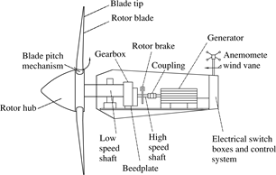
Basically, the wind turbine transforms the energy of air mass movement into electrical energy. The electromechanical model of the wind turbine depends on the parameters related to the aerodynamics and the size of the generator. In order to allow the maximum power extraction, it is necessary to obtain the most accurate mathematical model in order to implement an appropriate MPPT control. The most relevant variables involved are the nominal speed of the turbine, the gearbox ratio, the electromagnetic torque of reference, the pitch angle, and the TSR [11], [12], [13]. In Fig. 1, a description of the basic elements of a wind turbine is detailed.
Aerodynamic Model
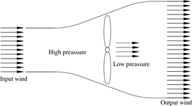
Aiming to produce the movement of the wind turbine rotor, the air enters the swept rotor area which is a circumference created by the rotation of the blades. The rotor captures the energy of the air, causing a decrease of pressure once the energy is transferred to the mechanism of the wind turbine detailed in Fig. 2 [7].
The aerodynamic model represents the energy extraction of the rotor, and calculates the mechanical torque as a function of the air flow in each propeller. The wind speed can be considered as the average speed of the incident wind in the area swept by the propellers with the purpose of evaluating the average torque in the low speed axis [5]. The mechanical power can be determined by the expression in equation (1) [1], [3], [14].

However, the wind turbine can recover only part of available power because of the Betz limit shown in (2). Here is where the term Cp affects the wind turbine performance due to mechanical and electrical losses.

Where, R is the wind turbine blade radius, ρ is the air density, V v is the wind speed, and Cp is the power coefficient.
For a wind turbine, Betz's law establishes that 59.26% of the kinetic energy of the wind can be converted into useful mechanical energy [7]. The other losses of the system described by the parameter Cp are defined by the relationship in (3).

For a wind turbine, Cp is, on a regular basis, experimentally by the manufacturers. The Cp depends on TSR and pitch angle β described in equation (4). The general equation (5) makes reference to the family of curves that relates TSR to Cp of a wind turbine [7], [13].


Where

Mechanical Model
For the mechanical model, the two-mass representation of the speed joint in the power transmission and linked to the gearbox which transmits the torque caused by the impact of the wind has been modeled in this work. The mechanical model is displayed in Fig. 3.
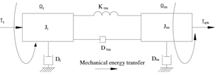
The left side of Fig. 3 represents the low-speed part, where the propellers are generating the low-speed rotational movement. On the right, the high-speed side which is attached to the generator rotor is located. The moment of inertia and torque are detailed in equations (7) [5], [7].

Where:
The model can be simplified by discarding the damping coefficients (Dt, Dm, and Dtm); hence, resulting in a two-inertia model (Jt and Jm) and the stiffness constant (Ktm).
Pitch Control Model
The objective of the controller is to manipulate the pitch of the propellers at different angles to increase or decrease the wind turbine speed. The β-pitch controllers allow independent control of each propeller usually through hydraulic actuators. This permits the reduction of the tension generated in the entire system. Pitch angle regulation is modeled, as shown in Fig. 4, by a PI controller which generates a reference rate. This reference is limited, and a first order system provides the dynamic behavior of the speed control of the wind variation. The angle of inclination itself is then obtained by integrating the variation of the angle. The control of a variable-speed wind turbine is needed to calculate both the generator torque and the pitch angle references in order to comply with the generator speed regulation [7].

Wind Turbine Speed Control
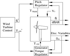
The wind turbine benchmark is oriented to design high power systems (1 MW onwards). For such applications, DFIGs are popular as they can generate high controllable power thanks to the size of the power electronics converters compared to other wind turbine technologies [7], [15]. For instance, it can be seen, in Fig. 5, a general control scheme for the operation of the Wind Turbine at variable speed, where there are two important input signals for the controllers: the generator electromagnetic reference torque and the pitch angle command.
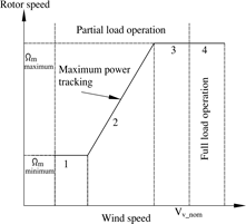
The main goal is to extract the maximum energy from the wind, keep the wind turbine in a safe operating mode (power, speed and torque below limits), and mechanical stress reduction on the drivetrain. The turbine control operation zones used in the development of this work is illustrated in Fig. 6 and consists of four areas of operation [7] where four zones are displayed: 1) Minimum operating speed zone restriction, 2) MPPT zone into partial load operation for variable speed operation until nominal speed is achieved, 3) the maximum speed in partial load operation and 4) full load operation before the brake is applied. The objective of the proposed controllers is to regulate the operation of the wind turbine so that it works in its second operating zone, this will allow obtaining the maximum power monitoring.
INDIRECT SPEED CONTROL STRATEGY
The indirect speed control strategy is based on the relationship between the electromagnetic torque Tem and the angular velocity Ωt. Nonetheless, the relation between the electromagnetic torque and the angular velocity does not have a direct dynamic relationship due to the inertia involved. This leads to a much slower response of the system as the mechanical coupling is not canceled [7]. The ISC modifies the dq frame currents in order to command the back to back converter allowing the controllability of the slip angle which also affects the speed and torque of the generator. The scheme to be implemented is shown in Fig. 7.

When the wind turbine operates at optimal conditions, the parameters allow finding a constant value called k opt which is used for the optimal electromagnetic torque reference calculation. The general description can be found in equations (8). According to [7], the ISC can be achieved by measuring the LSS and subtracting the mechanical losses as shown in Figure. 7. The Electromagnetic torque of reference T em is calculated in terms of k opt and the LSS Ω m . In equation (9) and (10), it is shown how the k opt is determined. The ISC strategy also considers the mechanical losses at the gearbox established at block D including friction and damping factors [13], [16].


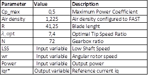
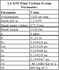
For k opt calculation it is necessary to establish the optimal TSR λ opt and the corresponding C p_max . These parameters can be either calculated experimentally or provided by the manufacturer. In this work, multiple simulations using Matlab and FAST where used to estimate λ opt , C p_max and compared to manufacturers specifications found in [17] (see Table 1).
Indirect Speed Control Implementation
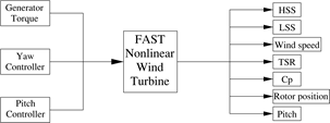
FAST models a wind turbine as a composition of rigid and flexible elements. For example, two-blade turbines are modeled as four rigid and four flexible bodies. The rigid bodies are the ground, the nacelle, the hub, and the tip brakes (point masses) whereas flexible bodies comprise blades, tower, and transmission system. The components of both flexible and rigid bodies include the following variables: tower bending, blade bending, nacelle yaw, rotor position, rotor speed, and driveshaft torsional flexibility. The tower bending has two modes, each in the front-to-back and side-to-side directions, and flexible blades have two modes of rotation and one edge per blade mode. In Fig. 8, the FAST model [18] implemented in Simulink [10] can be observed to obtain a matrix of output variables which directly interact in the proposed controller model.
For the implementation of the proposed control algorithm, the angular velocity at low speed is initially considered, and together with equation (10), the control block is carried out; thus, importing the variables calculated in FAST [8]. It is worth noting that the controller was designed in Matlab. The implementation of the control loop is observed in Fig. 9.
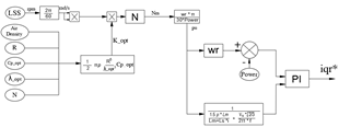
For the calculation of Iqr, which enters the PI control block, the expression (11) is used. This expression was calculated from the generated electromagnetic torque [3].

Where,
p = Generator pair of poles
SIMULATION RESULTS
ISC MPPT simulation strategy is based on a DFIG electric machine of 1,5MW output power at nominal speed. Some wind turbine parameters for FAST and Matlab configurations are displayed in Table 2. The ISC MPPT technique depends deeply on the dynamics of the system because the optimal constant calculated in equation (10) remains constant for all possible wind variations. The advantage of this method consists in its simplicity of implementation and conceptually it is easier to understand the response and calibrations over some parameters can be performed intuitively. This method requires precise characteristics of the wind turbine and evidently can be improved using Direct Speed Control (DSC) methods based on complex observers. It is important to note that ISC as well as DSC do not require to measure the wind for the control strategy. Instead, it can be calculated, predicted or estimated depending on the approach. Considering that dynamics of the wind turbine system and the corresponding MPPT ISC controller require to be tested at multiple wind conditions, three different wind speed signals were configured for analysis and validation. These signals where generated and imported to FAST where the outputs are calculated considering mainly partial load operations. The signals are generated considering different dynamic responses such as step, triangular and realistic functions. All the signals were created for evaluation purposes considering real ranges such as levels or slopes. Furthermore, there are some considerations for establishing the wind speed profiles. For instance, according to [7], the low speed region oscillates between 3,5 m/s and 5,5 m/s. Partial load operations where the MPPT ISC controller acts from a input wind speed of 5,5 to 11 m/s and the constant or nominal speed is established between 11 and 12 m/s. The Cp is plotted from time zero. Besides, the initial inertia, wind, and rotor speed cause the Cp to initiate in an unrealistic quantity; however, after ten seconds, the Cp swings between 0,4 and 0,5 which is desirable for this wind turbine (see Table 2). All the following experiments compare a traditional PID with the ISC controller.
Steady wind speed with ramp type transitions
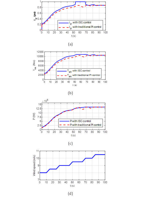
The first wind speed signal used for simulations consists of different levels of steady wind speed with ramp type transitions. The idea, here, is to provide a more deterministic signal to evaluate the controller response. It is well known that step shape functions are often used in order to determine the system response for drastic input variations. The wind speed input signal varies from 8 to 10 m/s and the plot can be observed in Fig. 10 (d). For the study`s purpose, 100 seconds of simulation have been tested. Thereon, the following outcomes were obtained. First, the output power remains about 1,275 MW in average. It is important to note that even though the wind turbine is at rated speed of 11 m/s, the simulation only considers the partial load. When the rated speed is attained, the output power reaches near 1,5MW, and these wind speed profiles generate a stable Cp near 0,5. In terms of the pitch controller, it also operates, but the simulations are intended to reduce its direct influence over the MPPT controller. In this test, the main achievement is the stability of the Cp signal in Fig. 10 (g), the ISC MPPT can be observed even though the Cp average value has short increase. However, the output power shown in Fig. 10 (c) also describes a small increment in level an also stability. Fig 10 (a) shows the Iq reference current in per units which is similar for both controllers, however, for the ISC the current is saturated between 50 and 70 seconds because the wind speed is over the partial load limit. For this experiment, pitch angle controller is activated when the magnitude of the wind is above 9,5 m/s which corresponds to the manufacturer specifications. The pitch angle can be observed in Fig. 10 (f) where the pitch angle executes three corrections before the steady state for traditional PI control and two corrections for the case of the ISC. This leads to a less pitch dependent approach reducing the stress of the components of the overall system.
Variable wind speed with positive and negative ramps
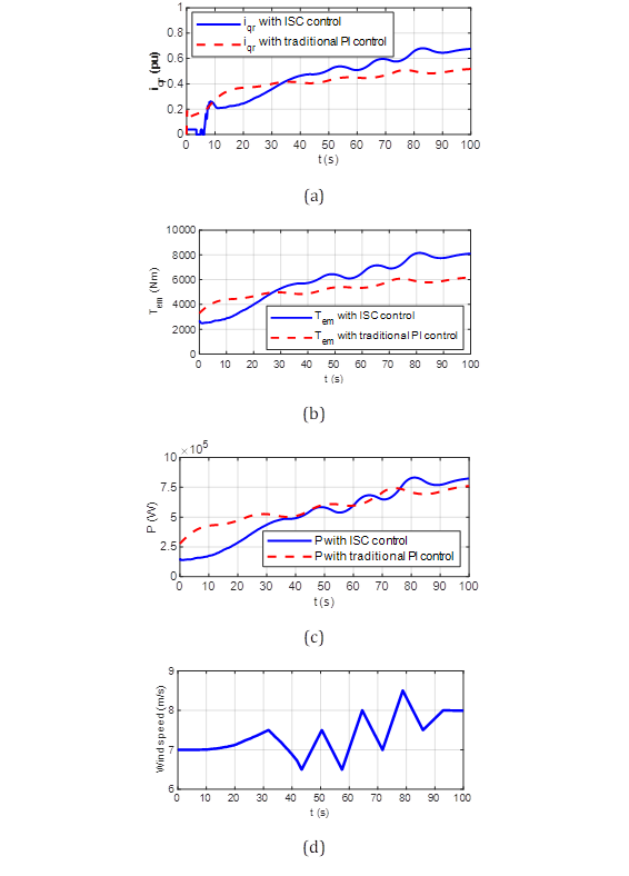
The second wind speed signal used for simulations consists of a variable wind speed with triangular type signal. The idea, here, is to test the system with a more realistic oscillatory signal in order to evaluate the dynamic response using triangular input winds. This signal simulates an increasing wind speed profile which varies between 6,5 and 8,5 m/s. To comply with the study`s guidelines, 100 seconds of simulation have been tested. The power remains about 0,9 MW in average during MPPT zone. It is fundamental to emphasize that even though the wind turbine has been configured at the rated speed of 11 m/s, the simulation is intended to evaluate the dynamic response during the variations of wind. Moreover, although the initial inertia and torque are low for testing the dynamics during partial load, a very strong oscillation at the beginning of the simulation which corresponds to the initial inertia configuration in FAST can be observed. When the rated speed is attained, the output power reaches near 0,75 MW, and the wind speed profiles generate a stable Cp near 0,5. With respect to the pitch controller, it also acts when the wind speed increases, and because of this, the system is tested mainly during partial load without a straight impact of pitch control. In Fig. 11 (a) it is shown the triangular input signal with small slopes stating with 7 m/s speed. For this experiments the pitch angle does not actually work because the wind speed is low as shown in Fig. 11 (f). The output power clearly increases after 80 seconds and remains higher for a steady state condition after 90 seconds as shown in Fig. 11 (c). Iqr displays smooth variations in Fig. 11 (a), however, it is able to produce changes also in the Cp which also has rapid variations following the response of the wind in the triangular shape function.
Variable Wind Speed with realistic input
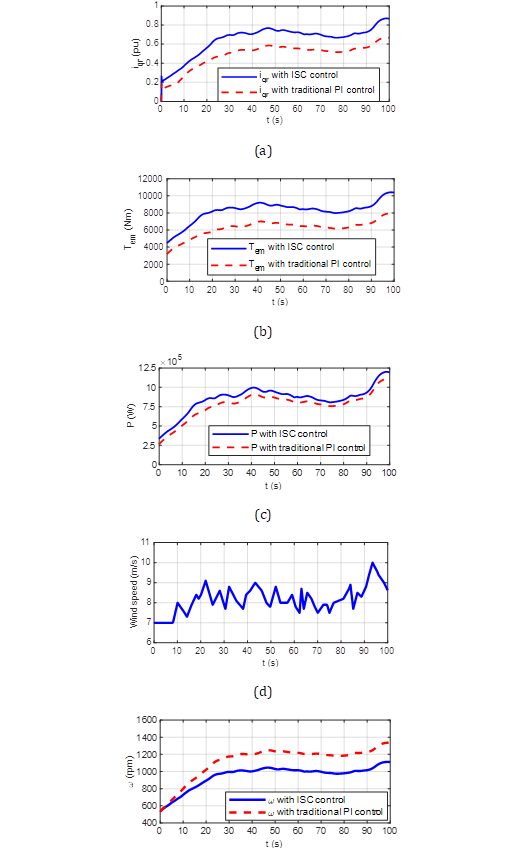
The third wind speed signal used for simulations consists of a variable wind speed with transitions. The idea, here, is to test the system with a more realistic oscillatory signal in order to evaluate the dynamic response. The oscillatory signal simulates an increasing wind speed profile which varies from 7 to 10 m/s. Thereupon, 100 seconds of simulation have been tested. Under those circumstances, the following results were obtained. First, the output power remains about 0,9MW in average during MPPT zone. At this instant, it is important to highlight that even though the wind turbine is at rated speed of 11 m/s, the simulation only considers the partial load and the initial conditions. Moreover, the initial inertia and torque are low for testing the dynamics during partial load. When the rated speed is attained, the output power reaches near 1,25MW due to the slip, and these wind speed profiles generate a stable Cp near 0,5. Regarding the pitch controller, it also acts when the wind speed increases, and because of this, the system is tested mainly during partial load without a straight impact of pitch control. The generated realistic input wind speed can be observed in Fig. 12 (d). The improvements of the Cp are observed in Fig. 12 (g) along basically all the curve. The pitch angle also remains zero because of the range of the wind speed as shown in Fig. 12 (f). Probably the best outcome during this experiment is the improvement of the output power along the curve following the variations of the inputted wind.
CONCLUSIONS
In this work, the ISC has been implemented by using FAST and Matlab for a DFIG 1,5MW wind turbine. Compared to the classical PI control, the results display an important improvement because of the correct selection of optimal TSR and maximum Cp when calculating the optimal constant at the controller stage. This implementation also considers the initial LSS speed and inertia which produce an oscillation during the first 20 seconds of simulation. Nevertheless, after that period of time, the rotor speed becomes steady and close to the nominal value. The aforementioned tests have the intention of demonstrating the capability of this technique for responding fast, even for disturbed wind input. Furthermore, the pitch control is able to perform a correct control for limiting the speed of the shaft. This is important since the Cp performance is also affected by the pitch angle. After the simulation enters a full load operation, the power and speed become nominal values, but in these experiments, the idea is to demonstrate the correct operation of the wind turbine along the partial load operation.
The DFIG electric machine could also have a different configuration for the connection to the grid; thus, allowing the system to provide more power depending on the active and reactive power. The ISC improvements compared with traditional PID controllers can be quantified in terms of stability but mainly of Cp maximization. This can be observed in the results when the average output active power is measured where the ISC allows more power extraction. Because of the nature of the wind turbine components, the dynamic error represents all possible stages of the wind turbine where the energy is transformed. The variations in the wind speed input produces many transients over the output power and power coefficient consequently. The wind speed is not usually constant for real scenarios and it is mostly considered as an oscillatory signal which produces a complex dynamic. The ISC could be improved when the knowledge of all possible variables is available since it is very sensitive to disturbances and implementation of DSC methods are recommended for better dynamic performance.

