Inglés (pdf)
 Articulo en XML
 Referencias del artículo
 Enviar articulo por email
 Citado por SciELO
  Similares en
SciELO
Similares en
SciELO 
 Permalink
Introduction
The constant evolution of technology has increased the need for better bandwidth and lower latencies, resulting in the rapid evolution of mobile systems. Since 1991 with the appearance of 2G, cellular networks have gained strength in our environment, being the only limitations bandwidths and cell sizes. Today, 2G networks are obsolete because of the high latencies and low data transmission they can provide; this is where technologies such as 3G and later 4G-LTE significantly improved the quality of service.
Nowadays, the next mobile generation system, called 5G NR (5th Generation Mobile Network - New Radio), has been released. Thus, it is important to understand the essential parts of the new 5G-NR standard and especially the parameters that intervene within the different scenarios of use in cell planning (Qualcomm, 2016). 5G-NR aims to surpass its predecessor, 4G-LTE technology, on many levels using higher frequencies and new network infrastructure. Its aim is to offer a superior service, being the high attenuation that occurs in signals at higher frequencies, the major challenge to overcome (Ahmadi, 2019).
The aim of 5G-NR is to have an NR access network and technology to satisfy a wide range of use cases, which are grouped into three main groups: Enhanced Mobile Broadband (eMBB), Massive Machine Type Communication (mMTC), and ultra-reliable and low latency communications (URLLC) (Otham, 2019). This grouping is based on the requirements detected for each case, such as capacity or latency (Pérez, 2019). It is important to mention that 5G-NR maintains both the signals and physical channels of its LTE predecessor, with certain variations, to provide greater operational flexibility. The basic unit of resources is the Physical Resource Block (PRB, made up of 12 consecutive sub-carriers. Its maximum number depends on the bandwidth and sub-carrier spacing as detailed in the 3GPP specifications (ETSI, 2021).
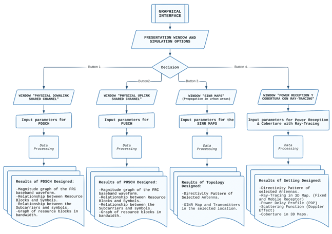
In this way, the standard proposes many configurations from which it is possible to proceed with the parameterization of 5G-NR channels and environments (ETSI, 2021). Once studied, it can be deployed within test environments in mathematical software such as MATLAB©, which provides the functions and the suitable environment for signal generation and data analysis (Mathworks, 2022). These simulations present different ways of planning for wireless technologies, which can serve as the basis for more complex and accurate models that can be implemented in the future to improve the software. The SINR maps considered the recommendations for urban cell planning proposed by the International Telecommunication Union (ITU, 2020), and research works that are already published on 5G propagation modeling (Rappaport, MacCartney, Samimi, & Sun, 2015; Samimi & Rappaport, 2016; Sulyman et al., 2014). The ray-tracing power reception and coverage section was based on ray-tracing principles (Yun & Iskander, 2015) and other propagation models like rain and fog (ITU, 2005, 2019). The presented software for network coverage analysis using MATLAB© tools and propagation modeling follows the operation flowchart detailed in figure 1.
This work also intends to expose interactively the basic planning guidelines for 5G-NR with an intuitive simulator that provides the option to experiment with parameters of transmission and behavior of gNodesB, as well as the use of the simulator made in MATLAB© ‘App Designer’ tool called “5G simulator for Urban Cell Planning”. This simulator was designed to be used by a student who can make their own designs and test them, which will help to increase the understanding of 5G-NR networks. Usually, these sorts of tools have a fee and cannot be given to users free of charge, which is why the development of this type of software that can be designed and subsequently distributed with no license is important in education and technology development, aim that was achieved with this research. The simulator presented in this paper focuses on its physical layer and can also help in planning urban cells through SINR maps (Signal to Interference & Noise Ratio) and Ray-Tracing simulations.
It is worth mentioning that 5G-NR infrastructure is already deployed in many countries around the world with several improvements (Guttman, 2017), and some authors (5G NR and Enhancements, 2022; Rinaldi, Raschellà, & Pizzi, 2021) emphasize the importance of its study and its technical features like its scalable numerology, ultra-lean and beam-centric design, support for low latency spectrum extension, among others. With this software, it will be possible to improve, facilitate and optimize the understanding of 5G technology and its planning, the latter being one of the main motivations for its development, besides delivering a useful and necessary tool to the students of the telecommunications career, thus generating a positive social impact. The simulator’s design was carried out based on the research and analysis of existing data on this technology provided by 3GPP and other organizations that contribute to its standardization. The main challenges involved defining and agreeing on the scope of the project, involving the end users from the beginning of the development, creating a concise and complete requirements document, confirming the understanding of the requirements, and creating a prototype to refine the final agreed-upon characteristics. Thus, contributing to the learning of anyone interested in this field, especially to students who are starting out in propagation and mobile communications, since along with the stand-alone version of the parameterizable simulator, technical memories, instructions, and virtual laboratory guides were also provided.
Finally, the software was exported and distributed to carry out an applicability test, with positive results regarding its functionality and ease of use. A comparison of results with a commercially available professional engineering tool was also carried out, which showed substantially similar coverage areas in both simulators.
The rest of the paper is organized as follows. Section 2 presents the methodology followed in the simulator’s development. Section 3 presents the results. Finally, sections 4 and 5 conclude the paper.
Methodology
Each of the procedures followed to carry out the parameterizable simulator were implemented using the parameters defined in the 3GPP standard as a basis, all of this to fulfill each of the initial objectives. First, the analysis of the 5G-NR information was carried out, for which a documentary investigation was used. Subsequently, the general specifications and properties were detailed, followed by the characteristics and functions used to make the parameterizable simulator to characterize its major components and present them in a user interface.
Once the functions to be used were defined, the parameterizable interface was developed within the mathematical software MATLAB©, which contains scripts developed and verified for the simulation of waves, radiation patterns and signal modulation, which can be analyzed and interpreted for later use. For the study of 5G-NR, the start point was a review of simulations and wave generation schemes to address them separately and determine the most important parameters to consider in planning.
Physical Downlink Shared Channel (PDSCH
For the parameterization of the Downlink, we analyzed the different sections of the standard. Here, only the FRCs (Fixed Reference Channels) will be considered, which are the channels with fixed characteristics. This type of information is quite useful, as the Physical Downlink Shared Channel parameters are used in several UE (User Equipment) tests, including:
• UE receiver requirements.
• UE maximum entry-level test.
Based on the standard, the first variable to choose will be the frequency band in which it will operate (table 1), since the options for the following parameters will be derived from this, such as the modulations used, the bandwidths, sub-carrier spacing, among others.
Table 1: Defined Frequency Ranges for 5G-NR.
| Frequency Range Designation | Corresponding Frequency Range |
|---|---|
| FR1 (Frequency Range 1) | 410MHz - 7125MHz |
| FR2 (Frequency Range 2) | 24250MHz - 52600MHz |
Once the Frequency Range has been determined, a bandwidth (BW) and a sub-carrier spacing (SCS) can be chosen to consider the combinations defined in the standard. Bearing in mind that, according to 3GPP, there are cases in which the combinations cannot be used and do not apply (ETSI, 2021), as for modulations, QPSK, 64QAM and 256QAM are used in the downlink FRCs (3GPP, 2020). Duplexing modes in 5G-NR are defined both in time and frequency, so FDD (Frequency Division Duplex) and TDD (Time Division Duplex) are used according to the specific needs of the channel to be configured. It is recommended that for transmission in paired and unpaired frequencies, FDD and TDD should be used, respectively.
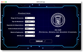
Once the parameters to be used in the PDSCH were studied and defined, the graphical interface was designed and programmed (figure 2). The parameterizable variables are presented as “Drop Down” containers. The containers are used to deliver the values to the user in accordance with the standard and automatically change the options that can be accessed. That is, changing one parameter will influence others, and the interface will automatically adapt to this change.
Physical Uplink Shared Channel (PUSCH
With the Physical Uplink Shared Channel, there are types of channels well defined by the standard, called FRCs (Fixed Reference Channels) where, despite being fixed, they can be reconfigured in such a way as to provide some flexibility in the parameters, according to potential design needs. As in the PDSCH, the first variable to choose will be the frequency band in which it will operate, since we will derive the workable options for the following parameters from this, and it limits the bandwidths, sub-carrier spacing, and so on.
Once the frequency range has been determined, the bandwidth, sub-carrier spacing, and modulations such as QPSK, 16QAM and 64QAM can be chosen. Those parameters vary according to the type of FRC. The base properties were taken from the standard. It could be mentioned that in the uplink, it is appropriate to specify an N-cell-id (ETSI, 2021).
After the concepts were reviewed and the PUSCH parameters were defined, the graphical interface was designed in the development environment (figure 3), where the variables are presented sequentially as “Drop Down” containers. Similarly, containers are used to deliver the values to the user following the standard specifications.
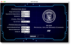
In the case of the PUSCH, the interface is arranged so that the user starts with the base parameters, and according to this, the software suggests a Fixed Reference Channel that meets the requested characteristics. The types of FRCs used as a base can later be modified with additional parameters, such as bandwidth, duplex mode, and the N-Cell-ID that will serve as the identifier of a cell.
Urban Planning - SINR Maps
The test environment guidelines for 5G technologies reuse the test network design of its 4G predecessor. Therefore, the guidelines are defined in Section 8.3 of the Report ITU-R M.2135-1(ITU, 2010), where in the rural/high-speed, urban coverage and micro-cell cases, specific topographical details are not considered.
The base stations are placed uniformly, following a hexagonal layout. In this hexagonal design, three cells are located per site, where the direction of the antenna, cell range and ISD (Inter-site Distance) are also defined. The simulation will be a surrounding configuration of 19 sites, each with three cells. Users are assumed to be dispersed throughout the area (ITU, 2010). The initial default values were taken from the ITU-R M.IMT-2020.EVAL (ITU, 2020).
The bandwidth and the rest of the remaining parameters depend on the usage scenario. For the Dense Urban-eMBB test environment, the default bandwidth is 20 MHz with the transmitted power of 44 dBm. The frequency designated for the test environment is 4 GHz, and the height defined for base stations is 25 meters, as detailed in (ITU, 2020, p. 18). However, the simulator allows changing those parameters.
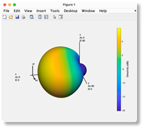
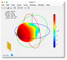
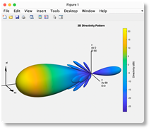
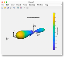
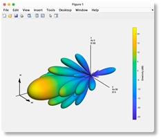
Also, different antenna radiation patterns can be used (figure 4 figure 5, figure 6, and figure 7). For each antenna pattern, a 3D graphic shows the directivity variation scale, intending to have a better idea of the antennas that are to be used in the simulations.
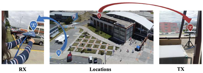
The entire map will be built based on the location of the central antenna, and from this, together with the ISD values, the network diagram will be built. Two test locations have been defined, which are in the center of Riobamba and the center of Quito. Additionally, different locations can be tested defining the longitude and latitude values in decimal degrees.
The graphical interface was designed as shown in figure 8. The containers are used to deliver the values that are necessarily fixed to the user, while the editable fields are configured with their default value. These parameters can be changed at the user’s discretion to experiment with different scenarios.
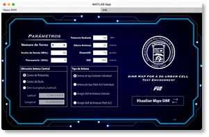
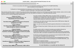
Also, to provide more information to the user, an information window was located, where the default parameters and some important aspects of the simulation can be verified, as shown in figure 9.
Parameters for Ray Tracing and Coverage
The proposed test environments for 5G use and consider different criteria from Report ITU-R M.2412 (ITU, 2021), which contains guidelines for the evaluation of radio interfaces for these technologies. After analyzing the physical structure of 5G-NR and the tentative SINR Maps, a deeper step would be conducted using the ray-tracing method.
Like in any telecommunications test environment, the basis will be the working frequency of the transmitter and receiver that will be displayed on a map, and from these, the corresponding calculations will be made. The main parameters considered are shown in table 2.
Table 2: Additional Parameters for Transmitters
| Name Property | Function |
|---|---|
| CoordinateSystem | Specify the coordinate system for the transmitter location, it can be defined as ‘geographic’ or ‘cartesian’. |
| Antenna | Specify antenna that will carry the transmitter, antennas created with the Phased Array System Toolbox™ can be used. |
| AntennaHeight | Height of the antenna from the ground or building surface, specified with a non-negative numeric scalar in meters. |
| AntennaAngle | Antenna x-axis angle defined regarding a local Cartesian coordinate system, specified as a numeric scalar representing an azimuth angle in degrees or as a 2-by-1 vector or 2-by-N matrix representing azimuth angles and elevation with each element unit in degrees. |
| TransmitterFrequency | Transmitter operating frequency, specified as a positive scalar in Hz. in the range [1e3 100e9]. |
| TransmitterPower | Signal power at the transmitter output, specified as a positive scalar in watts. The transmitter output is connected to the antenna. |
To construct a realistic scenario, the Site viewer tool was used, which allows importing external maps, such as the Open Street 3D building maps. These maps are created by a large community of people worldwide and are updated daily. Maps that can be downloaded from its own portal www.openstreetmap.org. These maps are the basis of the Ray Tracing simulator. With the imported map of the area of interest, transmitters or receivers can be placed and attribute their own characteristics. The MATLAB© antenna toolbox allows for creating sites and implementing antennas within the site viewer with different properties that can be modified in each item.
In the simulator’s case that was implemented, to calculate each of the reflections it is important to know the permittivities and conductivities of the external materials of the constructions and terrains, which can be calculated simply, as detailed in the ITU-R P.2040-1 recommendation (ITU, 2015). This equation is used to get the relative permittivity, where the calculated value depends on the working frequency and two constants:
Where a and b are constants characterizing the material, f is the frequency in GHz, and (' i’ dimensionless.
Physically, conductivity is interpreted as the facility offered by a material to establish a flow of electric current in it. According to their conductivity, materials are classified into conductors, semiconductors, and insulators. The international system (SI) units of conductivity are siemens/m. (Paz Parra, 2013). Equation (2) described in recommendation ITU-R P.2040-1 (ITU, 2015) was used to calculate the conductivity.
Being f the frequency in GHz and ( is expressed in S/m. The values of c and d are constants characterizing the material.
One of the most important steps in the calculations for free space loss (FSL) is to determine the losses in clear-sky conditions, as described in equation (3). These are the losses that remain constant, and the value of the distance can be obtained by the Ray-Tracing algorithm and together with the permittivity and conductivity at each reflection, a more accurate model can be obtained.
When the frequency f is represented in MHz and the distance d is in km.
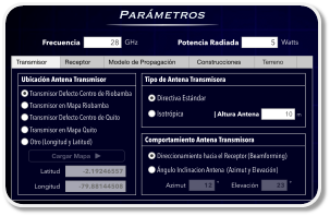
The location of the transmitter will be given in geographic coordinates, defined in their longitude and latitude. The height of the transmitter will depend on the test case; for the parameterizable simulator, an initial tower height value of 10 meters will be taken. The working frequency is a crucial point of the parameterizable simulator. The proposed software allows simulate the high frequencies used in 5G-NR; the default value is 28 GHz. The radiated power will depend on the user's approach and will be in Watts [W]. This parameter, like others, is left open to the user's criteria.
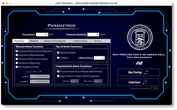
The types of antennas used can be generated from the same Phased Array System Toolbox™ that has integrated MATLAB software. A custom antenna from Report ITU-R M.2412, designated for the evaluation of 5G radio technologies, will be used in the simulator (ITU, 2021) (figure 10). An isotropic antenna was also used for more general tests, where all rays will be traced with the same gain in all directions.
For the simulator, an always fixed transmitter (gNodeB) was considered (figure 11). The antenna azimuth and elevation can be configured, which can be entered by the user or automatically assigned with the direction towards the receiver (beamforming mode).
There are likely scenarios in which there will be no LOS (Line of Sight) between the transmitter and the receiver. Here, the antenna will be directed at the angle of the ray with the slightest delay. In figure 12, the user interface is presented. Two preloaded maps of the city of Riobamba and Quito were integrated into the simulator, plus two default transmitter locations for test scenarios. However, it is possible to upload a map in ‘.osm’ format that can be downloaded from different web portals.
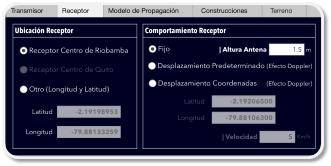
The 5G receiver UE (User Equipment) can be placed in any position on the map, and all reflections with power above the threshold of -120 dBm, will be considered. Also, the UE has 2 types of behaviors: i) Fixed Receiver and ii) Mobile Receiver (Doppler Effect). If it acts as a mobile receiver, the receiver’s coordinates must be entered, and additionally, the coordinates of the direction movement (figure 13). It allows the simulator to calculate the respective Doppler shift for each contribution.
While the empirical models are based on in situ measurements, the theoretical models are based on the fundamental principles of electromagnetic wave propagation phenomena. The propagation models predict the loss that can occur along the path that a radio frequency signal follows, between a base station and one or more receivers (UE) that can be fixed or mobile (Camargo, 2009). The SBR (shooting and bouncing rays) algorithm is a hybrid method that combines PO (Physical Optics) and Geometrical Optics (OG). Electromagnetic propagation is first represented by optical rays’ reflection, refraction, and divergence. Millions of ray tubes are launched from the source to the scatterer, and the paths of each ray tube bouncing off the scatterer’s surfaces are plotted according to Snell’s law. Next, the electromagnetic properties of magnitude, direction, and phase are added to the ray traces to mimic the properties of waves. Then, the contribution of each ray tube to the stray field is calculated independently. Finally, the scatterer under the irradiation of the incident wave can be expressed as the superposition of the individual contributions of all the ray tubes (Xu, Dong, Zhao, Yin, & Chen, 2021).
For a more intuitive use of the software, three switches were used, as shown in figure 14, one for each propagation model incorporated in the simulator, where the ‘Ray-Tracing SBR’ model will be activated by default. Besides this, it will be possible to activate rain models (ITU, 2005) or mist (ITU, 2019).
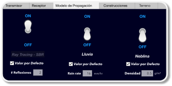
Recommendation ITU-R P.840-8 provides methods to predict attenuation because of clouds and fog, considering that it is necessary to give guidelines to engineers for the design and simulation of telecommunication systems in frequencies higher than 10 GHz. Clouds and fog are composed entirely of tiny droplets, generally less than 0.01 cm, so the Rayleigh approximation is valid for frequencies up to 200 GHz; the specific attenuation inside a cloud or fog is expressed in dB/Km (ITU, 2019). For the use of this fog and cloud propagation model within the parameterizable simulator, the working frequency of the transmitter and an extra parameter of the density of liquid water in the fog will be necessary, by default, it will be 0.5 g/m^3.
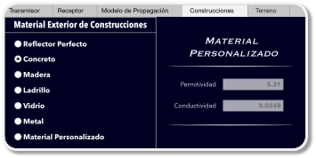
With the implemented simulator, to calculate each one of the reflections, it is important to know the permittivity of the exterior materials of the constructions, which can be calculated merely, as detailed in the recommendation ITU-R P.2040-1 (ITU, 2015).
The graphical interface of the exterior material for the constructions is designed so that one of the materials described can be chosen (figure 15). In addition, a custom material can be entered, defined by its permittivity and conductivity. This process is carried out analogously for terrain materials.
Once the parameters of the transmitter, receiver, and a propagation model have been defined, they can be combined with functions such as ‘coverage’. This function performs the computation as for a point, but in a particular area, considering the same attributes of each one of the elements. The button to generate the coverage graphic is also at the same interface. The last window with all the functions to the user is shown in figure 16.
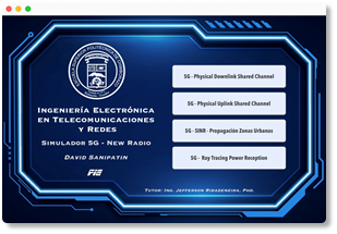
The general graphic interface (figure 17) contains the cover and four buttons that access each of the mentioned parts of the project. It allows a single window of each type to be opened at a time, and when it is closed, all windows derived from it are closed.
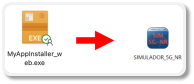
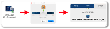
Finally, the parameterizable simulator was exported as an autonomous executable or ‘standalone’ for Windows and Mac OS (figure 18), and a MATLAB application (figure 19), being the distribution formats to the end users. These versions can be used for free, under the agreements specified by MathWorks®.
Results
After the consolidation of the software, multiple tests were carried out in each scenario to evaluate its behavior and on-site measurements for comparison with real results. Also, a survey was also carried out to determine the perspective of the simulator’s operation by the end users and its potential benefits.
Physical Downlink Shared Channel
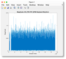
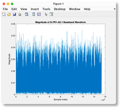
After the parameters are adjusted at the user’s discretion, the software will design the channel. In this case, the first to appear is figure 20, which is the magnitude of the FRC baseband waveform. The values of each of the samples are generated to satisfy the chosen options, and thus complete all the resource blocks.
These samples, after going through the post-process, can be displayed as Resource Blocks, where the relationship of the symbols concerning their use is represented by colors. These blocks can be designated for the PDCCH (Physical downlink control channel), PDSCH, Coreset (Control resource set) or SS Burst (Synchronization signal burst). The length frame in 5G is 10 ms for FDD and 20 ms for TDD. Each frame comprises 10 subframes, and these subframes comprise their respective Slots, which will depend on the chosen numerology. With 30KHz, each 1 ms subframe comprises 2 slots of 14 OFDM symbols. An easy way to calculate the number of total symbols per 1ms subframe would be by multiplying the number of Slots defined in the numerology multiplied by the 14 OFDM symbols that make up each slot. A total of 280 symbols on the X-axis is obtained, as shown in figure 21.
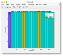
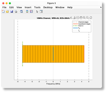
Figure 22 illustrates the frequency bandwidth to be used, centered at 0 Hz and having the channel edges in dotted lines. The channels must have guard bands that are shown in red; the center point of the resource blocks is represented by 𝑘 0 and the center frequency by 𝑓 0 .
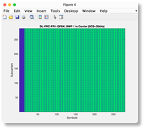
Each RB (Resource Block) is made up of 12 Sub-carriers. Therefore, the total number of Sub-carriers will be 288, having a maximum of 24 RBs for the chosen configuration. The relationship between each of the symbols and the Sub-carriers can be seen in figure 23.
Physical Uplink Shared Channel
In the case of the PUSCH, the interface is arranged so that the base parameters are entered first, and according to this, the software will suggest an FRC that adapts to the user's requirements.
Additionally, the interface has additional parameters, which can be changed at the discretion of each user and will be helpful for testing. Figure 24 illustrates the relationship between magnitude and the symbols that will be entered into the resource blocks.
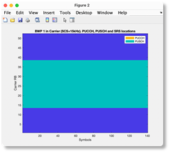
For the chosen base FRC 'G‘F‘1-A2-1',’t’e standard states that there will have a total of 25 occupied RBs, which is why figure 25 shows only 25 occupied of the 52 total.
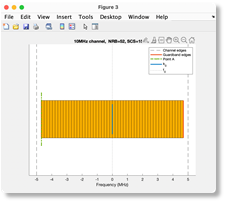
Figure 26 depicts the maximum number of RBs that can be accommodated within the guard bands of the selected bandwidth. The center point of the resource blocks is represented by 𝑘 0 and the center frequency by 𝑓 0 .
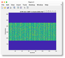
Figure 27 shows the relationship between the Subcarriers and the symbols of the chosen configuration. Note that the dark blue ones are not hosted blocks, and in the case of the blue ones that are inside the channel, they work as pilot symbols.
SINR maps for urban cell planning
As an example, a specific simulation using the parameters detailed in table 3 was performed.
Table 3: Simulation Parameters SINR Maps.
| Location Central Tower (Downtown Riobamba) | ||
|---|---|---|
| Longitude | -1.672823 | |
| Latitude | -78.648214 | |
| Cell Parameters for SINR Map | ||
| Number of Towers | 19 | |
| I.S.D. | 200 meters | |
| Downtilt | 15 degrees | |
| Antenna Height | 25 meters | |
| Transmission Parameters for SINR Map | ||
| Antenna Type | Single Standard Antenna | |
| Work Frequency | 4GHz | |
| Channel Bandwidth | 20MHz | |
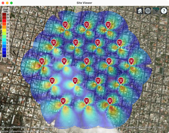
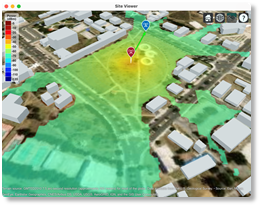
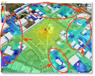
In this case, when choosing the type of antenna, the radiation pattern of the chosen option will be displayed. After the parameters of table 3 were simulated, the distribution of the towers in the center of the city of Riobamba is shown as in figure 28, and it is visualized that since it is not such a directional antenna, the SINR tends to be lower.
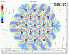
In the ‘topographic map’ type view, there is a better appreciation of the coverage area of the cells. Figure 29 presents a simulation made with the standard 8x8 antenna. Because of the antenna has better directivity, it can be seen how the cells and the area have better reception C/I, compared with figure 28.
Ray Tracing in urban cells
A specific scenario inside the “ESCUELA SUPERIOR POLITÉCNICA DEL CHIMBORAZO (ESPOCH)” was simulated. Table 4 presents the simulation parameters.
Table 4: Simulation Parameters for Ray Tracing
| Transmission Parameters | |||
|---|---|---|---|
| Frequency | 28GHz | ||
| Radiated Power (Ptx) | 5 Watts | ||
| Transmitter Parameters (ESPOCH - Riobamba) | |||
| Longitude | -1.657267 | ||
| Latitude | -78.677692 | ||
| Antenna Height | 10 meters | ||
| Antenna Type | Standard Directive | ||
| Transmitter Behavior | Beamforming | ||
| Receiver Parameters (ESPOCH - Riobamba) | |||
| Longitude | -1.656363 | ||
| Latitude | -78.677459 | ||
| Antenna Height | 1.5 meters | ||
| Antenna Type | Isotropic - 0dB | ||
| Receiver Behavior | Fixed | ||
| Propagation Models | |||
| Ray Tracing SBR | State | ON | |
| Max. reflections | 3 | ||
| Rain | State | ON | |
| Rain Rate | 16mm/hr | ||
| Fog | State | ON | |
| Density | 0.5g/m3 | ||
| Materials | |||
| Building Material | ‘Concrete’ | ||
| Ground Material | ‘Loam’ | ||
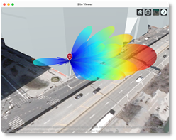
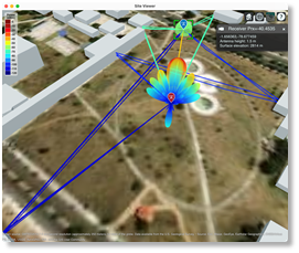
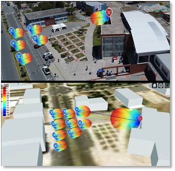
In the simulation, the radiation patterns of both the transmitter and the receiver are displayed. The names of the elements and their properties are shown when clicked, including the received power, coordinates, and the antenna height, as can be seen in figure 30.
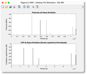
Also, the graph of the PDP (Power Delay Profile) is shown, where each one of the rays received by the UE is characterized. In the upper graph of the figure 31, the power received from each of the rays are represented, and in the lower graph, is shown the normalized and excess delay PDP that arrives at the receiver.
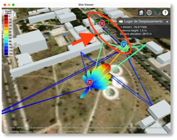
In the second case, where the receiver has movement, each element can be viewed in the ‘Site Viewer’. As can be seen in figure 32, the direction is represented with a blue arrow towards a second location called ‘Place of Displacement’.
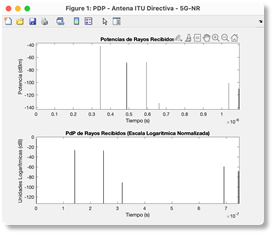
Similarly, the PDP graph is shown, where each one of the rays received by the UE is characterized (figure 33). In the upper graph of the figure, the received power and the delay of each ray is represented, and in the lower graph, the PDP normalized to the first traced ray that reaches the receiver.
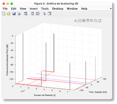
With a mobile receiver advancing towards the ‘Place of Displacement’ at 5 Km/h, will cause the so-called ‘Doppler Effect’, which causes a shift in the frequency components to higher or lower frequencies, depending on the angle of arrival of the corresponding ray. Figure 34 shows the shifts in frequency produced by the movement of the receiver, represented in the Scattering function.
Coverage in urban cells
For coverage, the same Ray Tracing criteria are considered, but in a particular area. As can be seen in figure 35, the transmitter, receiver model and coverage footprint are represented on the map, as well as an arrow between the transmitter and receiver model to verify LOS.
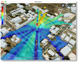
Figure 36 presents the coverage map for the same case shown in figure 35, but with a single reflection. It can be seen the improvement in the reception area since more reflections were considered. These show the importance of reflections, especially in urban environments.
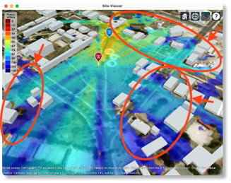
As mentioned above, the same ray-tracing criteria are considered for coverage, but in a particular area. In figure 36, the simulation of a transmitter with an isotropic antenna can be observed.
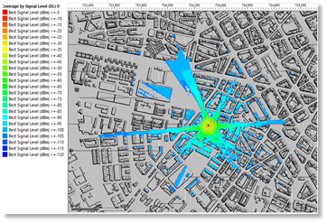
In the case of 10 reflections with the isotropic antenna (figure 37) and (figure 38) a better coverage can be seen in all directions and an increased power, even in not so accessible places; this because of the more significant number of contributions that will exist for each point.
Comparison with a professional simulation tool
As part of the applicability evaluation, the parameterizable simulator was contrasted with other software on the market, which is an advanced engineering tool that provides multiple options for planning and designing cellular networks. Table 5 shows the parameters used for the comparison.
Table 5: Simulation Parameters for the Comparison.
| Transmission Parameters | ||
|---|---|---|
| 5G-NR Parameterizable Simulator | Professional simulation tool V3.3.0.7383 | |
| Frequency | 2.8GHz | 2.8GHz |
| Radiated Power (Ptx) | 5 Watts | 5 Watts |
| Calculation distance | 600 meters. | 600 meters |
| Transmitter Parameters (Valencia - Spain) | ||
| Longitude | 39.4641119 | 39.4641119 |
| Latitude | -0.3939393 | -0.3939393 |
| Antenna Height | 10 meters | 10 meters |
| Antenna Type | Isotropic | Isotropic |
| Antenna Gain | 0dB | 0dB |
| Receiver Parameters (Valencia - Spain) | ||
| Longitude | 39.4642037 | 39.4642037 |
| Latitude | -0.39417317 | -0.39417317 |
| Antenna Height | 1.5 meters | 1.5 meters |
| Antenna Type | Isotropic - 0dB | N/A |
| Receiver Behavior | Permanent | Permanent |
| Propagation Model | ||
| Propagation Model Name | ‘Ray-Tracing SBR’ | ‘Standard Model’ |
| Reflections | 10 | N/A |
| Materials | ||
| Building Material | ‘Concrete’ | N/A |
| Ground Material | ‘Concrete’ | N/A |
One model in the professional simulation tool is the standard propagation model, which is a model deduced from the Hata formula, and from which various studies confirm that it is a very suitable model for UMTS, CDMA2000, WiMAX and LTE, so it will be able to work at the test frequency of 2.8 GHz (Popoola, 2017). In the case of the proposed parameterizable simulator, it will work with the Ray Tracing SBR propagation model that can perform the calculation for up to 10 reflections in any building scenario imported in 3D.
As can be seen in figure 39, the professional simulation tool also allows the use of propagation models that adapt to the needs of a user, being able to locate both transmitting and receiving antennas, and displaying results within the map. In the version of the professional simulation tool in which the simulations were carried out, there is no specific model for 5G, nor a ray-tracing propagation model, for which a frequency that fits in the FR2 of 5G was used for comparisons.
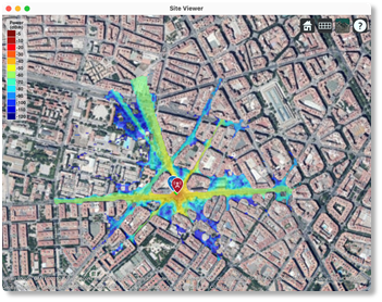
Figure 40 shows that the simulator generates similar results to professional simulation tools. Therefore, the simulator proposed applies for basic planning environments. In addition, it could be also used for education through the designed laboratory guides and support documents.
In situ measurements
Complementary to the development of the simulator, measurements in situ were taken. In the scenario, two Hyperlog antennas were used, an Anritsu MS2427C spectrum analyzer for the receiver, an Anritsu MG3690C signal generator besides cables and connectors. The collected data was helpful to know the difference between the simulations carried out and the measurements. The same geo-referenced locations were used in the simulator and in the measurement places. The proposed scenario is displayed in figure 41.
This test scenario was established with a frequency of 5.9 GHz and a transmission power of 18 dBm, a system loss margin of 10 dBm was set and the antennas have around 5 dBi gain. For the simulator, similar radiation patterns to real antennas were used, as shown in figure 42.
Once the samples were taken at the geo-referenced locations, they were compared with each of the results obtained at the same coordinates within the simulator.
Table 6: Parameters of the Test.
| LOCATION | MEASURED VALUE | SIMULATED VALUE | DIFFERENCE |
| Location 1 | -74.43 dBm | -66.4993 dBm | +7.93 dBm |
| Location 2 | -71.62 dBm | -64.8059 dBm | +6.81 dBm |
| Location 3 | -74.35 dBm | -67.6598 dBm | +6.69 dBm |
| Location 4 | -73.43 dBm | -66.3365 dBm | +7.09 dBm |
| Location 5 | -71.23 dBm | -65.8842 dBm | +6.35 dBm |
| Location 6 | -75.76 dBm | -68.8369 dBm | +6.92 dBm |
| Location 7 | -75.02 dBm | -67.7268 dBm | +7.29 dBm |
| Location 8 | -74.27 dBm | -67.3562 dBm | +6.91 dBm |
| Location 9 | -75.40 dBm | -67.3562 dBm | +8.04 dBm |
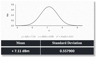
The measurement and simulated results are presented in table 6, getting a difference of between +6.35 dBm and +8.04 dBm between the measurements and the results obtained by simulation, with a mean difference of +7.11 dB and standard deviation of 0.5579 (figure 43). Showing that the results are quite suitable for urban planning environments, considering that differences between calculated and measured values are inferior to in other popular propagation models, like those evaluated by Sharma & Singh (2010).
Applicability Survey
After the consolidation of the simulator, a qualitative survey focused on evaluating its applicability and collecting the points of view of the users was applied. This survey was carried out by 24 students of the subject of mobile communications belonging to the ESPOCH Telecommunications career. The technique used was the Likert Scale with five possible answers, from strongly agree to strongly disagree. The estimated completion time was 4 minutes.
The survey results showed that the users strongly agreed that the use of simulations is a valuable teaching method for learning, where 75% said they strongly agreed and 25% agreed.
Respondents from their level of knowledge perceive that the scenarios where the simulations are developed are close to reality, with 71% of respondents agreeing and 29% strongly agreeing. Showing that the use of 3D maps and visual resources helps to improve the understanding and interpretation of results.
There was a strongly positive response, since the students felt they could apply previously gained knowledge to experiment with the simulator. Having 54% of those surveyed agree and 38% strongly agree with this idea. Along with other results that helped to improve the software and reflected that students of these topics have a great interest in simulated environments as a complement to theory.
Discussion
The analysis of the 5G-NR technology at the link and wave generation level was carried out, thus identifying its main characteristics, which were useful to focus the simulator on the most essential parts, being the PDSCH, PUSCH, SINR maps and the ray-tracing using the SBR method, the components that were implemented within the parameterizable simulator. The parameterization of the PDSCH and PUSCH based on the FRCs proposed in the standard allows users to experiment with the different configurations, which can be changed automatically at the interface according to the case. There are also some concerns such as the uncertainty of synchronization signals in the frequency domain and the flexibility of frame structure configuration, which are major challenges for the initial search of cells for the new fifth generation (5G) radio that this work does not consider and are detailed in (Chen, Li, Zhang, & Jiang, 2020) .
Planning scenarios in urban areas were implemented through programming in MATLAB-App Designer, the first was through SINR maps with a cellular network topology, which is a significant beginning, but real-world applications will have to consider some deployment challenges as those discussed in (Ahamed & Faruque, 2021), and the second one, using Ray-Trancing in 3D maps for urban cell planning that would be useful to know the final coverage, but to improve the analysis could also be considered other methods such as those described in (Carneiro de Souza, de Souza Lopes, de Cassia Carlleti dos Santos, Cerqueira Sodré Junior, & Mendes, 2022) for indoor environments, or another computer-based propagation tool based in (Erceg, Fortune, Ling, Rustako, & Valenzuela, 1997). The current techniques (Fuschini, Vitucci, Barbiroli, Falciasecca, & Degli-Esposti, 2015) in these ray-tracing tools allow to overcome traditional high CPU time limitations while the higher operating frequency makes ray-optics approximations less drastic and allows to achieve an unprecedented level of accuracy. This implies that having this tool exported would give the user the possibility of having a powerful design tool in their hands without having to pay a license fee.
Each one can be applied in realistic OSM maps, providing flexibility to the user’s requirements and the possibility of experimenting with different parameters.
The results show that the parameterizable simulator can be used in the teaching-learning process as an important tool for students and new professionals in the area, and also as a suitable tool in urban planning because of the simplicity of its characteristics. Now, this simulator is used by students of the Escuela Superior Politecnica de Chimborazo, where was evaluated and presented as one of the last results of the ‘N2MMWAVES’ Investigation Project. Feel free to email the authors if you want access to the simulator.
Conclusions
The parameterization of the PDSCH and PUSCH based on FRC proposed in the standard allows users to experiment with the different configurations which can be changed according to the case. On the other hand, there is the urban cell planification with SINR maps and Ray-Tracing which allows the user to have a general perspective of the planification and the topology. To evaluate the behavior of the simulator, a comparison was made with another simulation tool for engineering and an applicability survey to students, both reflected good results towards its performance, and even served as feedback to improve the software.
To evaluate the behavior of the simulator, a comparison was made with a professional simulation tool, having a mean difference between the two of them of +7,11 dBm, showing its suitability for urban planning environments. Additionally, an applicability survey to students was carried out, reflecting good results towards its performance. This software is closed to changes, but the development could be continued by the research groups of the Escuela Superior Politecnica de Chimborazo, where other projects based on the present work are being conducted.
Students have a great interest in simulated environments as a complement to theory, as showed the results of the survey, users strongly agreed that the use of simulations is a useful teaching method for learning where 75% indicated that they strongly agreed and 25% agreed. Respondents from their level of knowledge perceive that the scenarios where the simulations are developed are close to reality, 71% of respondents agreeing and 29% strongly agreeing. The students also felt that they could apply previously gained knowledge to experiment with the simulator, having 54% of those surveyed agree and 38% strongly agree.
This tool exported would give the user a powerful design tool, without having to pay a license fee. These kinds of simulators can be developed in different programming environments and that would serve as a guide not only for students but also for professionals who want training in a certain area. The software was distributed together with laboratory practices so that observations can be recorded, and in this way, be used in the teaching of topics such as propagation and mobile communications.
Acknowledgments
This paper and the research behind it would not have been possible without the exceptional support of the Escuela Superior Politecnica de Chimborazo (ESPOCH) and the National Secretariat of Higher Education, Science, Technology, and Innovation (SENESCYT).
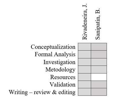
Authors’ contributions
In accordance with the internationally established taxonomy for assigning credits to authors of scientific articles (https://casrai.org/credit/). The authors declare their contributions in the following matrix: