Introduction

This paper is devoted to prove the exact controllability of a semilinear retarded equations under the influence of infinity delay, impulses and nonlocal conditions; verifying once again the conjecture that says: The controllability is preserve under the influence of delay, impulses and nonlocal conditions if some conditions are assumed. Specifically, we shall prove that the controllability of the associated time dependent linear systems is preserve by the following semilinear retarded system of differential equations with impulses, infinite delays, and nonlocal conditions:

where 0< 𝑡 1 < 𝑡 2 <⋯< 𝑡 𝑝 <𝜏, 0< 𝜏 1 < 𝜏 2 <…< 𝜏 𝑞 <𝜏, are fixed real numbers, 𝑧(𝑡)∈ ℝ 𝑛 , 𝑢(𝑡)∈ ℝ 𝑚 , 𝑧 𝑡 is defined as a function from (−∞,0] to ℝ 𝑛 by 𝑧 𝑡 (𝑠)=𝑧(𝑡+𝑠),−∞<𝑠≤0, 𝒜(𝑡), ℬ(𝑡) are continuous matrices of dimension 𝑛×𝑛 and 𝑛×𝑚 respectively, the control function 𝑢 belongs to 𝐿 2 ([0,𝜏]; ℝ 𝑚 ), 𝒟: ℌ 𝑞 →ℌ , with ℌ being a particular phase space satisfying the axiomatic theory defined by Hale and Kato (which will be specified later), 𝜑∈ℌ, ℎ:[0,𝜏]×ℌ× ℝ 𝑚 → ℝ 𝑛 , 𝒥 𝑘 ∈𝐶( ℝ 𝑛 × ℝ 𝑚 ; ℝ 𝑛 ), 𝑘=1,2,3,…,𝑝, such that

with 0<𝜂≤1, 0< 𝛼 𝑘 ≤1, 0< 𝛽 𝑘 ≤1, 𝑘=0,1,2,3,…,𝑝, and

Next, we will define the space of normalized piecewise continuous function, denoted by 𝒞 𝒜 𝑝 =𝒞 𝒜 𝑝 ((−∞,0]; ℝ 𝑛 ), as the set of functions such that their restriction to any interval of the form [𝑎,0] is a piecewise continuous function. i.e.,

Adapting some ideas from ^{Hale & Kato (1978}), ^{Liu (2000}) and Liu, Naito, & Van Minh (2003), we confider the function 𝑑:ℝ→ ℝ + satisfying the following conditions:

Remark 1.1. For example, we can consider the function 𝑑 as 𝑑(𝑠)=𝑒𝑥𝑝(−(−𝑠), with 𝑎>0.

The following spaces will be defined in order to set our problem

Lemma 1.2. The space 𝒞 𝑑𝑝 equipped with the norm

turns out to be a Banach space.

So, the phase space for our problem will be

together with the norm

Next, we are going to consider the following bigger space

defined by

As a consequence of Lemma 1.2, we get the following result

Lemma 1.3. 𝒞 𝒜 𝑑𝜏 is a Banach space endowed with the following norm

where 𝑧 | 𝐼 ∞ = 𝑠𝑢𝑝 𝑡∈𝐼=(0,𝜏] 𝑧(𝑡) .

Due to the fact that the function 𝑑 is defined on the entire real line, we can prove the following lemma satisfying axiom A1)-iii) from Hale and Kato axiomatic theory for the phase space. This Lemma play an important role in the prove of our main result.

In the same way, the following spaces are defined

ℌ 𝑞 =ℌ×ℌ×⋯×ℌ= 𝑖=1 𝑞 ‍ ℌ

∥𝑧 ∥ 𝑞 = 𝑖=1 𝑞 ‍ ∥ 𝑧 𝑖 ∥ ℌ

Also, we are going to use the following spaces

𝒞 𝒜 𝑑𝜏 ((−∞,𝜏]; ℝ 𝑛 )×𝐶([0,𝜏]; ℝ 𝑚 ),

with the norm

∥|(𝑧,𝑢)∥|=∥𝑧 ∥ 𝒞 𝒜 𝑑𝜏 +∥𝑢 ∥ 0 .

For a given (𝑧,𝑢)∈𝒞 𝒜 𝑑𝜏 ((−∞,𝜏]; ℝ 𝑛 )×𝐶([0,𝜏]; ℝ 𝑚 ), we consider the following expression:

We consider the associated linear system to the semilinear system (1.1):

𝑧 ′ (𝑡)=𝒜(𝑡)𝑧(𝑡)+ℬ(𝑡)𝑢(𝑡), 𝑡∈(0,𝜏], 𝑧(0)= 𝑧 0 . (1.6)

Next, the most important definition will be given, which is the definition of controllability for system (1,1):

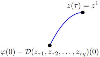
Definition 1.4 ( Controllability) If for every φ∈ℌ, z 1 ∈ ℝ n , there exists u∈C([0,τ]; ℝ m ) such that the solution z(t) of (1.1) verifies:

the system (1.1) is said to be controllable on [0,𝜏] figure 1.

figure 1: Controllability definition. 

One can find in the literature a large number of works on the controllability of linear systems (^{Chukwu, 1991}), including books, articles and monographs, see for example, Chukwu (1992), ^{Lee & Markus (1967}), and ^{Sontag (1998}). However, the references about the controllability of non-linear systems is limited, particularly for semilinear systems governed by differential equations, in this regard, we can refer to the article of ^{Lukes (1972}) and the book by ^{Coron (2007}) (see Theorem 3.40 and Corollary 3.41). On the other hand, ^{Vidyasager (1972}) proved the controllability for semilinear systems using Schauder’s Fixed Point Theorem and assuming that the non-linear term did not depend on the control u. Not so, ^{Dauer (1976}) found condition on semilinear systems that turns out to be weaker than the previous ones, which also allowed him to prove the controllability of such systems. But, ^{Do (1990}) weakened the previous conditions on the non-linear term and was able to prove the controllability of the semilinear systems; these new conditions generalize Dauer’s work; it is good to mention that these conditions strongly depend on the associated linear system (1.6) through its fundamental matrix; specifically the fundamental matrix Φ(𝑡) of the linear system 𝑧 ′ (𝑡)=𝒜(𝑡)𝑧(𝑡), which is in general not available in closed form. We must emphasize that in all these systems the influence of impulses, non-local conditions and delay is not taking into account.

There are many concepts of controllability depending on whether the control variable has restrictions, such as local controllability, which has been strongly studied by ^{Chukwu (1979}, 1980, 1987, 1991, 1992), ^{Mirza & Womack (1972}), ^{Sinha & Yokomoto (1980}), and Sinha (1985). But as far as we know, these studies are also not influenced by impulses, non-local conditions and delay, simultaneously, which is an open problem.

The controllability of differential equations with impulses, nonlocal condition and delay is at its peak at the moment, many mathematicians and engineers are devoted to the study of such equations; for example, for infinite dimensional systems governed by evolution equations, we can look at the works done by ^{Nieto & Tisdell (2010}) and ^{Zhu & Lin (2012}). Moreover, the work done in ^{Leiva (2014}a, 2014b) can be formulated in infinite dimension spaces. For infinite dimensional systems one can see ^{Selvi & Mallika (2012}), which studied the controllability of impulsive differential systems with finite delay by using measures of noncompactness and Monch’s Fixed Point Theorem. In Leiva (2014a, 2014b) the Rothe’s fixed point Theorem has been applied to prove the controllability of semilinear systems with impulses, which is the essential motivation for doing this work.

For infinite-dimensional Banach spaces, we are sure that some ideas presented here can be used to address also the controllability of evolution equations with impulses, delays, and nonlocal conditions simultaneously, and the nonlinear term involving all the variables, the time, the state , and the control. On the other hand, some results from ^{Carrasco, Leiva, Sanchez, & Tineo (2014}), Leiva (2014a), and Leiva & Merentes (2015) give us a good ideas to do this work.

In order to conclude this section, we will set the following result.

Lemma 1.5. For all function 𝑧∈𝒞 𝒜 𝑑𝜏 the following estimate holds for all 𝑠∈[0,𝜏]:

Theorem 1.6 (Rothe’s Fixed Theorem, (^{Banas & Goebel, 1980}; ^{Isac, 2004}; ^{Smart, 1980}) Let 𝐸 be a Banach space, and 𝐷⊂𝐸 be a closed convex subset such that the zero of 𝐸 is contained in the interior of 𝐷. Let 𝛹:𝐷→𝐷 be a continuous mapping with 𝛹(𝐷) relatively compact in 𝐸 and 𝛹(𝜕𝐷)⊂𝐷. Then, 𝛹 has at least a fixed point in 𝐷. i.e., There exists a point 𝑥 ∗ ∈𝐷 such that 𝛹( 𝑥 ∗ )= 𝑥 ∗ .

Our main hypotheses will be: The controllability of the linear system (1.6), the continuity of the fundamental matrix of the uncontrolled linear system and the conditions (1.2)-(1.5) satisfied by the nonlinear terms ℎ, 𝒟, 𝒥 𝑘 .

Controllability of Linear Systems

Now, we will give characterization for the controllability of linear systems (1.6) in the case when impulses, infinite delays and nonlocal conditions are not considered. In doing so, we shall consider, for all 𝑧 0 ∈ ℝ 𝑛 and 𝑢∈ 𝐿 2 ([0,𝜏]; ℝ 𝑚 ), the initial value problem

𝑧 ′ (𝑡)=𝒜(𝑡)𝑧(𝑡)+ℬ(𝑡)𝑢(𝑡), 𝑧∈ ℝ 𝑛 , 𝑡∈[0,𝜏], 𝑧(0)= 𝑧 0 , (2.1)

which admits only one solution given by

𝑧(𝑡)=𝒰(𝑡,0) 𝑧 0 + 0 𝑡 ‍ 𝒰(𝑡,𝑠)ℬ(𝑠)𝑢(𝑠)𝑑𝑠, 𝑡∈[0,𝜏], (2.2)

with given by 𝒰(𝑡,𝑠)=Φ(𝑡) Φ −1 (𝑠), where Φ(𝑡) is the fundamental matrix of the following corresponding differential equation

𝑧 ′ (𝑡)=𝒜(𝑡)𝑧(𝑡). (2.3)

i.e., the matrix Φ(𝑡) verifies:

Φ ′ (𝑡)=𝒜(𝑡)Φ(𝑡), Φ(0)= ?? ℝ 𝑛 , (2.4)

where 𝐼 ℝ 𝑛 is the 𝑛×𝑛 identity matrix. Hence, there exist constants Ω>0 and 𝜔>0 such that

∥𝒰(𝑡,𝑠)∥≤Ω 𝑒 𝜔(𝑡−𝑠) ≤𝑀, 0≤𝑠≤𝑡≤𝜏. (2.5)

Definition 2.1. Associated with system (1.6) the following linear operators are defined: The controllability operator (for τ>0) 𝒢: L 2 ([0,τ]; ℝ m )⟶ ℝ n is defined as follows

𝒢𝑢= 0 𝜏 ‍ 𝒰(𝜏,𝑠)ℬ(𝑠)𝑢(𝑠)𝑑𝑠. (2.6)

he adjoint operators 𝒢 ∗ : ℝ 𝑛 ⟶ 𝐿 2 ([0,𝜏]; ℝ 𝑚 ) of the operator 𝒢 is given by

𝒢 ∗ 𝑧 𝑠 = ℬ ∗ 𝑠 𝒰 ∗ 𝜏,𝑠 𝑧, ∀𝑠∈ 0,𝜏 , ∀ 𝑧∈ ℝ 𝑛 (2.7)

and the Controllability Gramian operator 𝒲: ℝ 𝑛 → ℝ 𝑛 is given by

𝒲𝑧=𝒢 𝒢 ∗ 𝑧= 0 𝜏 ‍ 𝒰(𝜏,𝑠)ℬ(𝑠) ℬ ∗ (𝑠) 𝒰 ∗ (𝜏,𝑠)𝑧𝑑𝑠. (2.8)

Proposition 2.2. The systems (6) is controllable on [0,𝜏] if, and only if, 𝑅𝑎𝑛(𝒢)= ℝ 𝑛 .

Also, we will use the following result from ^{Curtain & Pritchard (1978}) and Curtain & Zwart (1995).

Lemma 2.3. Let 𝑌 and 𝑍 be Hilbert space, 𝒢∈𝐿(𝑌,𝑍) and 𝒢 ∗ ∈𝐿(𝑍,𝑌) the adjoint operator. Then the following statements holds,

(i) 𝑅𝑎𝑛(𝒢)=𝑍⇐∃𝛾>0 / ∥ 𝒢 ∗ 𝑧 ∥ 𝑊 ≥𝛾∥𝑧 ∥ 𝑍 , 𝑧∈𝑍.

(ii) 𝑅𝑎𝑛(𝒢) =𝑍⇐ker( 𝒢 ∗ )={0}⇐ 𝒢 ∗ 𝑖𝑠 1−1.

Lemma 2.4. Then the following claims are equivalent

Hence, the maps Υ: ℝ 𝑛 → 𝐿 2 ([0,𝜏]; ℝ 𝑚 ) given by

Υ𝑧= ℬ ∗ (⋅) 𝒰 ∗ (𝜏,⋅) 𝒲 −1 𝑧= 𝒢 ∗ (𝒢 𝒢 ∗ ) −1 𝑧, (2.9)

is called the steering operator and it is a right inverse of 𝒢, which means that

𝒢Υ=𝐼. (2.10)

Moreover,

∥ 𝒲 −1 𝑧∥=∥(𝒢 𝒢 ∗ ) −1 𝑧∥≤ 𝛾 −1 ∥𝑧∥, 𝑧∈ ℝ 𝑛 , (2.11)

and a control steering the system (6) from initial state 𝑧 0 to a final state 𝑧 1 at time 𝜏>0 is given by

Lemma 2.5. (^{Leiva, 2014}b) Let 𝒯 be any dense subspace of 𝐿 2 ([0,𝜏]; ℝ 𝑚 ). Then, system (6) is controllable with control 𝑢∈ 𝐿 2 ([0,𝜏]; ℝ 𝑚 ) if, and only if, it is controllable with control 𝑢∈𝒯. i.e.,

𝑅𝑎𝑛(𝒢)= ℝ 𝑛 ⇐𝑅𝑎𝑛(.𝒢 | 𝒯 )= ℝ 𝑛 ,

where .𝒢 | 𝒯 is the restriction of 𝒢 to 𝒯.

Remark 2.6. Due to the previous Lemma, if the linear system (1.6) is controllable, it is controllable with control functions in the following dense subspaces of L 2 (0,τ; ℝ m ):

𝒯=𝐶([0,𝜏]; ℝ 𝑚 ), 𝒯= 𝐶 ∞ ([0,𝜏]; ℝ 𝑚 ), 𝒯=𝒞𝒜([0,𝜏]; ℝ 𝑚 ).

Moreover, the operators 𝒢, 𝒲 and Υ are well defined in the space of continuous functions: 𝒢:𝐶([0,𝜏]; ℝ 𝑚 )⟶ ℝ 𝑛 by

𝒢𝑢= 0 𝜏 ‍ 𝒰(𝜏,𝑠)ℬ(𝑠)𝑢(𝑠)𝑑𝑠, (2.13)

and 𝒢 ∗ : ℝ 𝑛 ⟶𝐶([0,𝜏]; ℝ 𝑚 ) by

( 𝒢 ∗ 𝑧)(𝑠)= ℬ ∗ (𝑠) 𝒰 ∗ (𝜏,𝑠)𝑧, ∀𝑠∈[0,𝜏]. ∀𝑧∈ ℝ 𝑛 . (2.14)

Also, the Controllability Gramian operator still the same 𝒲: ℝ 𝑛 → ℝ 𝑛

𝒲𝑧=𝒢 𝒢 ∗ 𝑧= 0 𝜏 ‍ 𝒰(𝜏,𝑠)ℬ(𝑠) ℬ ∗ (𝑠) 𝒰 ∗ (𝜏,𝑠)𝑧𝑑𝑠. (2.15)

Finally, the operators Υ: ℝ 𝑛 →𝐶([0,𝜏]; ℝ 𝑚 ) defined by

Υ𝑧= ℬ ∗ (⋅) 𝒰 ∗ (𝜏,⋅) 𝒲 −1 𝑧= 𝒢 ∗ (𝒢 𝒢 ∗ ) −1 𝑧, (2.16)

is a right inverse of 𝒢, in the sense that

𝒢Υ=𝐼. (2.17)

Results

In this part, we will prove the controllability of the nonlinear system (1.1) with impulses, infinite delays, and nonlocal conditions. To do so, for all 𝜑∈ℌ and 𝑢∈𝐶([0,𝜏]; ℝ 𝑚 ), due to ^{Leiva (2018}), the initial value problem

𝑧 ′ (𝑡)=𝒜(𝑡)𝑧(𝑡)+ℬ(𝑡)𝑢(𝑡)+ℎ(𝑡, 𝑧 𝑡 ,𝑢(𝑡)), 𝑡∈(0,𝜏],𝑡≠ 𝑡 𝑘 𝑧(𝑠)+𝒟( 𝑧 𝜏 1 , 𝑧 𝜏 2 ,…, 𝑧 𝜏 𝑞 )(𝑠)=𝜑(𝑠), 𝑠∈(−∞,0], 𝑧( 𝑡 𝑘 + )=𝑧( 𝑡 𝑘 − )+ 𝒥 𝑘 (𝑧( 𝑡 𝑘 ),𝑢( 𝑡 𝑘 )), 𝑘=1,2,3,…,𝑝, (3.1)

has one solution given by

𝑧 𝑢 (𝑡)=𝒰(𝑡,0){𝜑(0)−𝒟( 𝑧 𝜏 1 , 𝑧 𝜏 2 ,…, 𝑧 𝜏 𝑞 )(0)}+ 0 𝑡 ‍ 𝒰(𝑡,𝑠)ℬ(𝑠)𝑢(𝑠)𝑑𝑠 (3.2)

+ 0 𝑡 ‍ 𝒰(𝑡,𝑠)ℎ(𝑠, 𝑧 𝑠 𝑢 ,𝑢(𝑠))𝑑𝑠

+ 0< 𝑡 𝑘 <𝑡 ‍ 𝒰(𝑡, 𝑡 𝑘 ) 𝒥 𝑘 (𝑧( 𝑡 𝑘 ),𝑢( 𝑡 𝑘 )), 𝑡∈[0,𝜏].

𝑧(𝑡)=𝜑(𝑡)−𝒟( 𝑧 𝜏 1 , 𝑧 𝜏 2 ,…, 𝑧 𝜏 𝑞 )(𝑡), 𝑡∈(−∞,0].

Now, we define the following nonlinear operator

given by the formula:

where Θ 1 and Θ 2 are given as follow:

And

such that:

And

With

The following proposition follows trivially from the definition of the operator Θ.

Proposition 3.1. The Semilinear System (1.1) with impulses, infinite delay, and nonlocal conditions is controllable if, and only if, for all initial state φ∈ℌ and a final state z 1 the operator Θ given by ^{Leiva & Zambrano (1999}), ^{Liu (2000}) and Liu et al. (2003) has a fixed point. i.e.,

∃ 𝑧,𝑢 ∈𝐷𝑜𝑚 Θ 𝑠𝑢𝑐ℎ 𝑡ℎ𝑎𝑡 Θ 𝑧,𝑢 = 𝑧,𝑢 .

Theorem 3.2. Suppose that conditions (1.2)-(1.5) hold and the linear system (1.6) is controllable on [0,𝜏]. If 0≤ 𝛼 𝑘 <1, 0≤ 𝛽 𝑘 <1, 𝑘=0,1,2,3,…,𝑝, 0≤𝜂<1, then the nonlinear system (1.1) is controllable on [0,𝜏]. Moreover, exists a control 𝑢∈𝐶([0,𝜏]; ℝ 𝑚 ) such that for a given 𝜑∈ℌ, 𝑧 1 ∈ ℝ 𝑛 the corresponding solution 𝑧 𝑢 (⋅) of (1.1) satisfies:

𝑧 1 =𝒰(𝜏,0){𝜑(0)−𝒟( 𝑧 𝜏 1 , 𝑧 𝜏 2 ,…, 𝑧 𝜏 𝑞 )(0)}+ 0 𝜏 ‍ 𝒰(𝜏,𝑠)ℬ(𝑠)𝑢(𝑠)𝑑𝑠

+ 0 𝜏 ‍ 𝒰(𝜏,𝑠)ℎ(𝑠, 𝑧 𝑠 𝑢 ,𝑢(𝑠))𝑑𝑠+ 0< 𝑡 𝑘 <𝜏 ‍ 𝒰(𝜏, 𝑡 𝑘 ) 𝒥 𝑘 ( 𝑡 𝑘 ,𝑧( 𝑡 𝑘 ),𝑢( 𝑡 𝑘 )),

and

𝑢(??)= ℬ ∗ (𝑡) 𝒰 ∗ (𝜏,𝑡) 𝒲 −1 ℒ(𝑧,𝑢),

With

− 0< 𝑡 𝑘 <𝜏 ‍ 𝒰(𝜏, 𝑡 𝑘 ) 𝒥 𝑘 (𝑧( 𝑡 𝑘 ),𝑢( 𝑡 𝑘 )).

Proof. We shall prove this theorem by claims.

Statement 1. The operator Θ is continuous. In fact, to prove the continuity of Θ, it is enough to prove the continuity of the operators Θ 1 and Θ 2 defined above.

The continuity of Θ 1 follows from the continuity of the nonlinear functions ℎ(𝑡, 𝑧 𝑠 ,𝑢), 𝒥 𝑘 (𝑧,𝑢), 𝒟(𝑧) and the following estimate

∥ Θ 1 (𝑧,𝑢)− Θ 1 (𝑤,𝑣)∥≤ 𝐾 1 ∥𝑧−𝑤∥

+ 𝐾 2 sup 𝑠∈𝐽 ∥ℎ(𝑠, 𝑧 𝑠 ,𝑢(𝑠))−ℎ(𝑠, 𝑤 𝑠 ,𝑣(𝑠))∥|

+ 𝐾 3 0< 𝑡 𝑘 <𝑡 ‍ ∥𝒥 𝐽 𝑘 ( 𝑡 𝑘 ,𝑧( 𝑡 𝑘 ),𝑢( 𝑡 𝑘 ))− 𝒥 𝑘 ( 𝑡 𝑘 ,𝑤( 𝑡 𝑘 ),𝑣( 𝑡 𝑘 ))∥,

where,

𝐾 1 = 𝐾 4 𝐾 , 𝐾 2 = 𝑀 𝑤 𝐾 , 𝐾 3 = 𝑀 3 𝐾 , 𝑤𝑖𝑡ℎ 𝐾 =1+ 𝑀 2 𝜔 ∥ℬ ∥ 2 ∥ 𝒲 −1 ∥,

and 𝐾 4 = 𝑀 3 𝐾.

The continuity of the operator 𝒮 2 follows from the continuity of the operators ℒ and Υ define above.

Statement 2. 𝒮 maps bounded sets of 𝒞 𝒜 𝑑𝜏 ((−∞,𝜏]; ℝ 𝑛 )×𝐶([0,𝜏]; ℝ 𝑚 ) into equicontinuous sets of 𝒞 𝒜 𝑑𝜏 ((−∞,𝜏]; ℝ 𝑛 )×𝐶([0,𝜏]; ℝ 𝑚 ).

Consider the following equality

∥Θ(𝑧,𝑢)( 𝑡 2 )−Θ(𝑧,𝑢)( 𝑡 1 ) ∥ 1 =∥ Θ 1 (𝑧,𝑢)( 𝑡 2 )− Θ 1 (𝑧,𝑢)( 𝑡 1 )∥

+∥ Θ 2 (𝑧,𝑢)( 𝑡 2 )− Θ 2 (𝑧,𝑢)( ?? 1 )∥

Let 𝐷⊂𝒞 𝒜 𝑑𝜏 ((−∞,𝜏]; ℝ 𝑛 )×𝐶([0,𝜏]; ℝ 𝑚 ) be a bounded set. The equicontinuity for Θ(𝐷) is given by the equicontinuity of each one of its components Θ 1 (𝐷), Θ 2 (𝐷), which are obtained from the continuity of 𝒰(𝑡,𝑠) and the following estimates ∀(𝑧,𝑢)∈𝐷

Since 𝒰(𝑡,𝑠) is continuous ∥𝒰( 𝑡 2 ,𝑠)−𝒰( 𝑡 1 ,𝑠)∥ goes to zero as 𝑡 2 → 𝑡 1 and so does the sum and the integral from 𝑡 1 to 𝑡 2 , which implies that Θ 1 (𝐷) is equicontinuous. Moreover, the equicontinuity of Θ 2 (𝐷) follows from the continuity of the evolution operator 𝒰(𝑡,𝑠). Hence, Θ maps bounded sets into equicontinuous sets.

Statement 3. The set Θ(𝐷) is relatively compact. Indeed, let 𝐷 be a bounded subset of 𝒞 𝒜 𝑑𝜏 ((−∞,𝜏]; ℝ 𝑛 )×??([0,𝜏]; ℝ 𝑚 ). By the continuity of ℎ, ℒ, and 𝒥 𝑘 , for ∀(𝑧,𝑢)∈𝐷 it follows that

where ∥ 𝒥 𝑘 (𝑧,𝑢)∥= sup 𝑡∈[0,𝜏] {∥ 𝒥 𝑘 (𝑧(𝑡,𝑢(𝑡)) ∥ ℝ 𝑛 } 𝑀 5 , 𝑀 6 , 𝒯 1 , 𝒯 2 ,…, 𝒯 𝑘 , ∈ℝ. Therefore, Θ(𝐷) is uniformly bounded. Now, we consider a sequence a { 𝜓 𝑖 =( 𝜓 1𝑖 , 𝜓 2𝑖 ):𝑖=1,2,…} in Θ(𝐷). Since { 𝜓 2𝑖 :𝑖=1,2,…} is contained in Θ 2 (𝐷)⊂𝐶([0,𝜏]; ℝ 𝑚 ) and Θ 2 (𝐷) is an uniformly bounded and equicontinuous family, by Arzelà-Ascoli Theorem we can assume, without loss of generality, that { 𝜓 2𝑖 :𝑖=1,2,…} converges. On the other hand, since { 𝜓 1𝑖 :𝑖=1,2,…} is contained in Θ 1 (𝐷)⊂𝒞 𝒜 𝑑𝜏 ((−∞,𝜏]; ℝ 𝑛 ), then . 𝜓 1𝑖 | (−∞,− 𝜏 𝑞 ] =𝜑−𝒟( 𝜑 𝜏 1 , 𝜑 𝜏 2 ,…, 𝜑 𝜏 𝑞 ), 𝑖=1,2,…. Taking into account that { 𝜓 1𝑖 :𝑖=1,2,…} is bounded and equicontinuous in [0, 𝑡 1 ], we can apply Arzelà-Ascoli Theorem to ensure the existence of a subsequence { 𝜓 1𝑖 1 :𝑖=1,2,…} of { 𝜓 1𝑖 :𝑖=1,2,…}, which is uniformly convergent on [0, 𝑡 1 ]. Now, consider the sequence { 𝜑 1𝑖 1 :𝑖=1,2,…} on the interval [ 𝑡 1 , 𝑡 2 ]. On this interval the sequence { 𝜓 1𝑖 1 :𝑖=1,2,…} is uniformly bounded and equicontinuous, and for the same reason, it has a subsequence { 𝜓 1𝑖 2 } uniformly convergent on [0, 𝑡 2 ]. In this way, for the intervals [ 𝑡 2 , 𝑡 3 ], [ 𝑡 3 , 𝑡 4 ], , [ 𝑡 𝑝 ,𝜏], we see that the sequence { 𝜑 1𝑖 𝑝+1 :𝑖=1,2,…} converges uniformly on the interval [0,𝜏].

Besides, in the interval [− 𝜏 𝑞 ,0] the function 𝜓 1𝑖 is piecewise continuous, then repeating the foregoing process we can assume that the subsequence { 𝜓 𝑖 𝑝+1 =( 𝜓 1𝑖 𝑝+1 , 𝜓 2𝑖 𝑝+1 ):𝑖=1,2,…} converges in Θ(𝐷). This means that Θ(𝐷) is compact, i.e., Θ(𝐷) is relatively compact.

Statement 4. for 0< 𝛼 𝑘 <1, 0< 𝛽 𝑘 <1, 𝑘=0,1,2,3,…,𝑝, 0<𝜂<1, the following limit holds.

where ∥|(𝑧,𝑢)∥|=∥𝑧 ∥ 0 +∥𝑢 ∥ 0 is the norm in the space 𝒞 𝒜 𝑑𝜏 ((−∞,𝜏]; ℝ 𝑛 )×𝐶([0,𝜏]; ℝ 𝑚 ).

Using the conditions (1.2)-(1.5), we get that

∥ℒ(𝑧,𝑢)∥≤

𝑀 1 + 𝑀 2 {𝑒∥𝑧 ∥ 𝜂 + 𝑎 0 ∥𝑧 ∥ 𝛼 0 + 𝑏 0 ∥𝑢 ∥ 𝛽 0 + 𝑐 0 }+ 𝑀 3 0< 𝑡 𝑘 <𝜏 ‍ { 𝑎 𝑘 ∥𝑧 ∥ 𝛼 𝑘 + 𝑏 𝑘 ∥𝑢 ∥ 𝛽 𝑘 + 𝑐 𝑘 },

Where

𝑀 1 =∥ 𝑧 1 ∥+ 𝑀 3 ∥𝜑(0)∥, 𝑀 2 = 𝑀 3 + 𝑀 𝜔 𝑎𝑛𝑑 𝑀 3 =𝑀 𝑒 𝜔𝜏 .

+∥ℬ∥ 𝑀 3 2 ∥ 𝒲 −1 ∥ 0< 𝑡 𝑘 <𝜏 ‍ { 𝑎 𝑘 ∥𝑧 ∥ 𝛼 𝑘 + 𝑏 𝑘 ∥𝑢 ∥ 𝛽 𝑘 + 𝑐 𝑘 }.

And

∥ Θ 1 (𝑧,𝑢)∥≤ 𝑀 3 ∥𝜑(0)∥+ 𝑀 2 𝜔 ∥ℬ ∥ 2 ∥ 𝒲 −1 ∥ 𝑀 1

+ 𝑀 2 𝐾 𝑒∥𝑧 ∥ 𝜂 + 𝑎 0 ∥𝑧 ∥ 𝛼 0 + 𝑏 0 ∥𝑢 ∥ 𝛽 0 + 𝑐 0

+ 𝑀 3 𝐾 0< 𝑡 𝑘 <𝜏 ‍ { 𝑎 𝑘 ∥𝑧 ∥ 𝛼 𝑘 + 𝑏 𝑘 ∥𝑢 ∥ 𝛽 𝑘 + 𝑐 𝑘 }.

Therefore,

≤ 𝑀 4 +{∥ℬ∥ 𝑀 3 𝑀 2 ∥ 𝒲 −1 ∥+ 𝑀 2 𝐾 }{𝑒∥𝑧 ∥ 𝜂 + 𝑎 0 ∥𝑧 ∥ 𝛼 0 + 𝑏 0 ∥𝑢 ∥ 𝛽 0 + 𝑐 0 }

+{∥ℬ∥ 𝑀 3 2 ∥ 𝒲 −1 ∥+ 𝑀 3 𝐾 } 0< 𝑡 𝑘 <𝜏 ‍ { 𝑎 𝑘 ∥𝑧 ∥ 𝛼 𝑘 + 𝑏 𝑘 ∥𝑢 ∥ 𝛽 𝑘 + 𝑐 𝑘 },

where 𝑀 4 is given by:

𝑀 4 = 𝑀 3 ∥𝜑(0)∥+∥ℬ∥∥ 𝒲 −1 ∥ 𝑀 1 { 𝑀 3 + 𝑀 2 𝜔 ∥𝐵∥}.

Hence,

∥|Θ(𝑧,𝑢)∥ |∥|(𝑧,𝑢)∥| ≤ 𝑀 4 ∥𝑧∥+∥𝑢∥

×{𝑒∥𝑧 ∥ 𝜂−1 + 𝑎 0 ∥𝑧 ∥ 𝛼 0 −1 + 𝑏 0 ∥𝑢 ∥ 𝛽 0 −1 + 𝑐 0 ∥𝑧∥+∥𝑢∥ }

+{∥ℬ∥ 𝑀 3 2 ∥ 𝒲 −1 ∥+ 𝑀 3 𝐾 }

× 0< 𝑡 𝑘 <𝜏 { 𝑎 𝑘 ∥𝑧 ∥ 𝛼 𝑘 −1 + 𝑏 𝑘 ∥𝑢 ∥ 𝛽 𝑘 −1 + 𝑐 𝑘 ∥𝑧∥+∥𝑢∥ } ,

Consequently,

Statement 5. The operator Θ has a fixed point. In fact, by Statement 4, we know that for a fixed 0<𝜌<1 there exists 𝑅>0 big enough such that

∥|Θ(𝑧,𝑢)∥|≤𝜌∥|(𝑧,𝑢)∥|, ∥|(𝑧,𝑢)∥|=𝑅.

Hence, if we denote by 𝐵(0,𝑅) the closed ball of center zero and radius 𝑅>0, we get that Θ(𝜕𝐵(0,𝑅))⊂𝐵(0,𝑅). Since Θ is a compact operator, Θ(𝐵) is relatively compact in 𝒞 𝒜 𝑑𝜏 ((−∞,𝜏]; ℝ 𝑛 )×𝐶([0,𝜏]; ℝ 𝑚 ), and maps the sphere 𝜕𝐵(0,𝑅) into the interior of the ball 𝐵(0,𝑅), we can apply Rothe’s fixed point theorem 1.6 to ensure the existence of a fixed point (𝑧,𝑢)∈𝐵(0,𝑅)⊂𝒞 𝒜 𝑑𝜏 ((−∞,𝜏]; ℝ 𝑛 )×𝐶([0,𝜏]; ℝ 𝑚 ) such that

Θ(𝑧,𝑢)=(𝑧,𝑢).

Hence, applying the Proposition 3.1, we get that the nonlinear system (1.1) is controllable on [0,𝜏]. Moreover,

𝑢=Υ𝔏(𝑧,𝑢)= ℬ ∗ (⋅) 𝒰 ∗ (𝜏,⋅) 𝒲 −1 𝔏(𝑧,𝑢),

such that for a given 𝜑∈ℌ, 𝑧 1 ∈ ℝ 𝑛 the corresponding solution 𝑧(𝑡)=𝑧(𝑡,𝑢) of (1.1) satisfies:

𝑧 1 =𝒰(𝜏,0){𝜑(0)−𝒟( 𝑧 𝜏 1 , 𝑧 𝜏 2 ,…, 𝑧 𝜏 𝑞 ))(0)}+ 0 𝜏 ‍ 𝒰(𝜏,𝑠)ℬ(𝑠)𝑢(𝑠)𝑑𝑠

+ 0 𝜏 ‍ 𝒰(𝜏,𝑠)ℎ(𝑠, 𝑧 𝑠 ,𝑢(𝑠))𝑑𝑠+ 0< 𝑡 𝑘 <𝜏 ‍ 𝒰(𝜏, 𝑡 𝑘 ) 𝒥 𝑘 ( 𝑡 𝑘 ,𝑧( 𝑡 𝑘 ),𝑢( 𝑡 𝑘 )).

It completes the proof.

Now, we present another version of the previous theorem, which follows from the estimates considered in Statement 4.

Theorem 3.3. Suppose the linear system (1.6) is controllable on [0,𝜏]. Then the nonlinear system (1.1) is controllable if one of the following statements holds:

and {∥ℬ∥ 𝑀 3 𝑀 2 ∥ 𝒲 −1 ∥+ 𝑀 2 𝐾 } 𝑏 0 <1.

and {∥ℬ∥ 𝑀 3 𝑀 2 ∥ 𝒲 −1 ∥+ 𝑀 2 𝐾 }( 𝑎 0 + 𝑏 0 )<1.

and {∥ℬ∥ 𝑀 3 𝑀 2 ∥ 𝒲 −1 ∥+ 𝑀 2 𝐾 }(𝑒+ 𝑎 0 + 𝑏 0 )<1.

and {∥ℬ∥ 𝑀 3 2 ∥ 𝒲 −1 ∥+ 𝑀 3 𝐾 } 𝑘∈ 𝑆 𝛼 ‍ 𝑎 𝑘 <1, where 𝑆 𝛼 ={𝑘: 𝛼 𝑘 =1}.

and {∥ℬ∥ 𝑀 3 2 ∥ 𝒲 −1 ∥+ 𝑀 3 𝐾 } 𝑘∈ 𝑆 𝛽 ‍ 𝑏 𝑘 <1, where 𝑆 𝛽 ={𝑘: 𝛽 𝑘 =1}.

and {∥ℬ∥ 𝑀 3 2 ∥ 𝒲 −1 ∥+ 𝑀 3 𝐾 }( 𝑘∈ 𝑆 𝛼 ‍ 𝑎 𝑘 + 𝑘∈ 𝑆 𝛽 ‍ 𝑏 𝑘 )<1, where

Proof Let us consider any of the conditions 𝑎)−𝑔). Then, from the estimates obtained in Statement 4, we get that

lim ∥|(𝑧,𝑢)∥|→∞ ∥|Θ(𝑧,𝑢)∥| ∥|(𝑧,𝑢)∥| <𝜌<1.

Hence, there exists 𝑅>0 such that

∥|Θ(𝑧,𝑢)∥|≤𝜌∥|(𝑧,𝑢)∥|, ∥|(𝑧,𝑢)∥|=𝑅.

Then, analogously to the previous theorem the proof of Theorem 3.3 immediately follows by applying Proposition 3.1.

Example

In this section, we present an example to illustrate our results. In this regard, we will apply Theorem 3.2 to the semilinear time dependent control system with impulses, delay and nonlocal conditions given by

where 𝒜(𝑡)=𝔞(𝑡)𝒜, ℬ(𝑡)=𝔟(𝑡)ℬ with 𝒜 and ℬ 𝑛×𝑛 and 𝑛×𝑚 constant matrices, respectively.

From ^{Leiva & Zambrano (1999}), if the Kalman’s rank condition holds true

𝑅𝑎𝑛𝑘[ℬ;𝒜ℬ;⋯; 𝒜 𝑛−1 ℬ]=𝑛,

then the following time dependent linear system

𝑧′(𝑡)=𝒜(𝑡)𝑧(𝑡)+ℬ(𝑡)𝑢(𝑡), 𝑡∈[0,𝜏]

with 𝒜(𝑡)=𝔞(𝑡)𝒜, ℬ(𝑡)=𝔟(𝑡)ℬ, is exactly controllable on [0,𝜏](^{Leiva & Zambrano, 1999}).

Here, the nonlinear terms and the impulsive functions are given as follows

𝑓(𝑡,𝜙,𝑢)= 3 ∥𝑢∥+1 ⋅ 3 𝜙 1 (− 𝑡 𝑝 ) 3 ∥𝑢∥+1 ⋅ 3 𝜙 2 (− 𝑡 𝑝 ) ⋮ ⋅ ⋮ 3 ∥𝑢∥+1 ⋅ 3 𝜙 𝑛 (− 𝑡 𝑝 ) ,

𝒟( 𝜑 1 , 𝜑 2 ,⋯, 𝜑 1 )= 𝑖=1 𝑞 ‍ 𝑠𝑖𝑛( 𝜑 𝑖1 ) 𝑠𝑖𝑛( 𝜑 𝑖2 ) ⋮ 𝑠𝑖𝑛( 𝜑 𝑖𝑛 ) ,

𝒥 𝑘 (𝑧,𝑢)=𝑐𝑜𝑠( ∥𝑢∥+1 ) 𝑠𝑖𝑛( 𝑧 1 𝑘 ) 𝑠𝑖𝑛( 𝑧 2 𝑘 ) ⋮ 𝑠𝑖𝑛( 𝑧 𝑛 𝑘 ) ,

Then

∥ℎ(𝑡,𝜑,𝑢)∥≤2 𝑛 ∥𝜑(− 𝑡 𝑝 )∥+2 ?? ∥𝑢∥+2 𝑛 ,

and since 𝒟 and 𝐽 𝑘 , 𝑘=1,2,⋯,𝑝 are bounded, the conditions (1.2)-(1.5) are satisfied. Hence, the system (29) is exactly controllable on [0,𝜏].

Final Remark

In this paper, we have proved that the controllability is robust in the presence of impulses, infinite delay, and nonlocal conditions. This happens for many real life control systems where impulses, delays, and nonlocal conditions are intrinsic phenomena of the system. Moreover, in several papers we have shown that the influence of impulses do not destroy the controllability of some known systems like the heat equation, the wave equation and the strongly damped wave equation (^{Carrasco et al., 2014}; ^{Leiva, 2014}b, 2015; Leiva & Merentes, 2015). Therefore, the same ideas presented in this work to prove the exact controllability can be used to prove the controllability of infinite dimensional systems in Hilbert spaces where the dynamical is given by the infinitesimal generator 𝐴 of a compact semigroup {𝑇(𝑡) } 𝑡≥0 , in this case we only get approximate controllability of the system.

Interest conflict

The funders had no role in the study design; in the collection, analysis or interpretation of data; in the writing of the manuscript or in the decision to publish the results.

Authors’ contributions

Following the internationally established taxonomy for assigning credits to authors of scientific articles (https://casrai.org/credit/). The authors declare their contributions in the following matrix: