


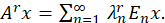
 Espanhol (pdf)
 Artigo em XML
 Referências do artigo
 Enviar este artigo por email
 Citado por SciELO
  Similares em
SciELO
Similares em
SciELO 
 Permalink
1 Introduction
There are several practical examples of control systems with impulses and delays: a chemical reactor system with the quantities of different chemicals serving as the state, a financial system with two state variables being the amount of money in a market and the saving rates of a central bank, and the growth of a population diffusing throughout its habitat, often modeled by reaction-diffusion equation. However, one may easily visualize situations in nature where abrupt changes such as harvesting, disasters, or instantaneous stoking may occur.
This paper has been motivated by the works done by Hugo Leiva in Leiva (2015a), Leiva (2015b), Leiva (2015c) where the approximate controllability of Semilinear Evolution Equation with impulses was proved in the case of non necessarily compact semigroup and bounded non linear perturbation.
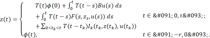
In this paper, we study a more general problem since we consider the following semilinear evolution equation with impulses and delays simultaneously
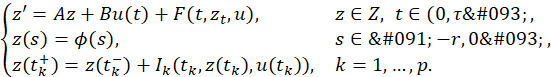
where 0< 𝑡 1 < 𝑡 2 < 𝑡 3 <⋯< 𝑡 𝑝 <𝜏, 𝑍 and 𝑈 are Hilbert Spaces,𝑢∈ 𝐿 2 (0,𝜏;𝑈), 𝐵:𝑈⟶𝑍 is a bounded linear operator, standard notation 𝑧 𝑡 defines a function from [−𝑟,0] to 𝑍 by 𝑧 𝑡 (𝑠)=𝑧(𝑡+𝑠),−𝑟≤𝑠≤0, 𝐼 𝑘 :[0,𝜏]×𝑍×𝑈→𝑍, 𝐹:[0,𝜏]×𝐶(−𝑟,0;𝑍)×𝑈→𝑍 are smooth functions, and 𝐴:𝐷(𝐴)⊂𝑍→𝑍 is an unbounded linear operator in 𝑍 which generates a strongly continuous semigroup {𝑇(𝑡) } 𝑡≥0 ⊂𝑍 non necessarily compact.
We assume the following hypotheses:
[(H1)]. The linear system without impulses (6) is approximately controllable on [𝜏−𝛿,𝜏] for all 0<𝛿<𝜏.
[(H2)]. The functions 𝐹, 𝐼 𝑘 smooth enough and
∥𝐹(𝑡,𝜙,𝑢) ∥ 𝑍 ≤𝑎∥𝜙(−𝑟)∥+𝑏,

Definition 1.1 (Approximate Controllability) The system (1) is said to be approximately controllable on [0,𝜏] if for every 𝜙∈𝐶(−𝑟,0;𝑍), 𝑧 1 ∈𝑍, 𝜀>0 there exists 𝑢∈ 𝐿 2 (0,𝜏;𝑈) such that the solution 𝑧(𝑡) of (1) corresponding to 𝑢 satisfies:
∥𝑧(𝜏)− 𝑧 1 ∥ 𝑍 <𝜀.
To address this problem we use a characterization dense range linear operator from Leiva et al. (2013), the approximate controllability of the linear equation on [𝜏−𝛿,𝜏] for all 𝜏>0 and the ideas presented in Bashirov et al. (2007), Bashirov & Ghahramanlou (2013) and Bashirov & Ghahramanlou (2014). The controllability of impulsive evolution equations has been studied recently by several authors, but most them study the exact controllability only, e.g. in Chalishajar (2011), studied the exact controllability of impulsive partial neutral functional differential equations with infinite delay, Radhakrishnan & Blachandran (2012) studied the exact controllability of semilinear impulsive integro-differential evolution systems with nonlocal conditions, and Selvi & Arjunan (2012) studied the exact controllability for impulsive differential systems with finite delay. To the best of our knowledge, there are a few works on approximate controllability of impulsive semilinear evolution equations, worth mentioning: Chen & Li (2010) studied the approximate controllability of impulsive differential equations with nonlocal conditions, using measure of noncompactness and Monch’s Fixed Point Theorem, and assuming that the nonlinear term 𝑓(𝑡,𝑧) does not depend on the control variable; Leiva & Merentes (2015) studied the approximate controllability of the semilinear impulsive heat equation using the fact that the semigroup generated by Δ is compact.
When it comes to the wave equation, the situation is totally different: the semigroup generated by the linear part is not compact; it is in fact a group, which can never be compact. Furthermore, if the control acts on a portion 𝜔 of the domain Ω for the spatial variable, then the system is approximately controllable only on [0,𝜏] for 𝜏≥2, which was proved by Leiva & Merentes (2010). More precisely, the following system governed by the wave equations was studied.
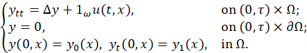
where Ω is a bounded domain in ℝ 𝑛 , 𝜔 is an open nonempty subset of Ω, 1 𝜔 denotes the characteristic function of the set 𝜔, the distributed control 𝑢∈ 𝐿 2 ([0,𝜏]; 𝐿 2 (Ω)) and 𝑦 0 ∈ 𝐻 2 (Ω)∩ 𝐻 0 1 , 𝑦 1 ∈ 𝐿 2 (Ω).
However, if the control acts on the whole domain Ω, it was proved in Larez et al., (2011) that the system is controllable [0,𝜏], for all 𝜏>0. More specifically, the authors studied the following system
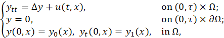
where Ω is a bounded domain in ℝ 𝑛 , the distributed control 𝑢∈ 𝐿 2 ([0,𝜏]; 𝐿 2 (Ω)) and 𝑦 0 ∈ 𝐻 2 (Ω)∩ 𝐻 0 1 , 𝑦 1 ∈ 𝐿 2 (Ω).
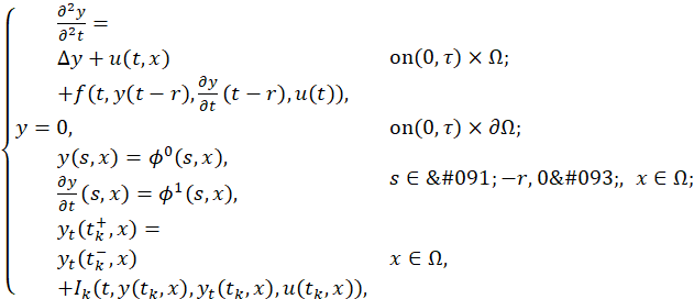
To justify the use of this new technique Bashirov & Ghahramanlou (2014), we consider as an application the following semilinear wave equation with impulses, delays and controls acting on the whole domain Ω, so that the hypotheses (H1) and (H2) hold:
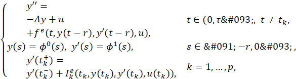
𝜕 2 𝑦 𝜕 2 𝑡 = Δ𝑦+𝑢(𝑡,𝑥) +𝑓(𝑡,𝑦(𝑡−𝑟), 𝜕𝑦 𝜕𝑡 (𝑡−𝑟),𝑢(𝑡)), on (0,𝜏)×Ω; 𝑦=0, on (0,𝜏)×𝜕Ω; 𝑦(𝑠,𝑥)= 𝜙 0 (𝑠,𝑥), 𝜕𝑦 𝜕𝑡 (𝑠,??)= 𝜙 1 (𝑠,𝑥), 𝑠∈[−𝑟,0], 𝑥∈Ω; 𝑦 𝑡 ( 𝑡 𝑘 + ,𝑥)= 𝑦 𝑡 ( 𝑡 𝑘 − ,𝑥) + 𝐼 𝑘 (𝑡,𝑦( 𝑡 𝑘 ,𝑥), 𝑦 𝑡 ( 𝑡 𝑘 ,𝑥),𝑢( 𝑡 𝑘 ,𝑥)), 𝑥∈Ω,
where 0< 𝑡 1 < 𝑡 2 < 𝑡 3 <…< 𝑡 𝑝 <𝜏, Ω is a bounded domain in ℝ 𝑛 , the distributed control 𝑢∈ 𝐿 2 ([0,𝜏]; 𝐿 2 (Ω)), 𝜙 0 ∈𝐶(−𝑟,0; 𝐻 2 (Ω)∩ 𝐻 0 1 ), 𝜙 1 ∈𝐶(−𝑟,0; 𝐿 2 (Ω)) and the nonlinear functions ??, 𝐼 𝑘 :[0,𝜏]×ℝ×ℝ×ℝ→ℝ are smooth enough and

2 Controllability of the Linear Equation
In this section we present some characterization of the approximate controllability of the corresponding linear equations without impulses and delays. To this end, we note that for all 𝑧 0 ∈𝑍 and 𝑢∈ 𝐿 2 (0,𝜏;𝑈) the initial value problem
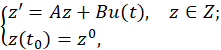
admits only one mild solution given by
𝑧(𝑡)=𝑧(𝑡, 𝑡 0 , 𝑧 0 ,𝑢)=

(See for example Curtain & Zwart (1995), Leiva (2003)).
Definition 2.1 For system (6) we define the following concept: The controllability map 𝐺 𝜏𝛿 : 𝐿 2 (𝜏−𝛿,𝜏;𝑈))→𝑍 defined by

The adjoint of this operator 𝐺 𝜏𝛿 ∗ :𝑍→ 𝐿 2 (𝜏−𝛿,𝜏;𝑈) is given by
( 𝐺 𝜏𝛿 ∗ 𝑧)(𝑡)= 𝐵 ∗ 𝑇 ∗ (𝜏−𝑡)𝑧, 𝑡∈[𝜏−𝛿,𝜏].
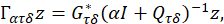
The Gramian controllability operators are given by:

The following lemma holds in general for a linear bounded operator 𝐺:𝑊→𝑍 between Hilbert spaces 𝑊 and 𝑍 (Bashirov et al.,2007, Leiva et al., 2013, Curtain & Pritchard, 2010, Curtain & Zwart, 1995).
Lemma 2.1 The following statements are equivalent to the approximate controllability of the linear system (6) on [𝜏−𝛿,𝜏]. [a)]
1. 𝑅𝑎𝑛𝑔𝑒( 𝐺 𝜏𝛿 ) =𝑍.
2. 𝐾𝑒𝑟( 𝐺 𝜏𝛿 ∗ )={0}.
3. 〈 𝑄 𝜏𝛿 𝑧,𝑧〉>0, 𝑧≠0 in 𝑍.
4. lim ??→ 0 + 𝛼(𝛼𝐼+ 𝑄 𝜏𝛿 ) −1 𝑧=0.
5. For all 𝑧∈𝑍, we have 𝐺 𝜏𝛿 𝑢 𝛼 =𝑧−𝛼(𝛼𝐼+ 𝑄 𝑇𝛿 ) −1 𝑧, where
𝑢 𝛼 = 𝐺 𝜏𝛿 ∗ (𝛼𝐼+ 𝑄 𝜏𝛿 ) −1 𝑧, 𝛼∈(0,1].
So, lim 𝛼→0 𝐺 𝜏𝛿 𝑢 𝛼 =𝑧 and the error 𝐸 𝜏𝛿 𝑧 of this approximation is given by the formula
𝐸 𝜏𝛿 𝑧=𝛼(𝛼𝐼+ 𝑄 𝜏𝛿 ) −1 𝑧, 𝛼∈(0,1].
6. Moreover, if we consider for each 𝑣∈ 𝐿 2 (𝜏−𝛿,𝜏;𝑈)) the sequence of controls given by
𝑢 𝛼 = 𝐺 𝜏𝛿 ∗ (𝛼𝐼+ 𝑄 𝜏𝛿 ) −1 𝑧+(𝑣− 𝐺 𝜏𝛿 ∗ (𝛼𝐼+ 𝑄 𝜏𝛿 ) −1 𝐺 𝜏𝛿 𝑣), 𝛼∈(0,1],
we get that:
𝐺 𝜏𝛿 𝑢 𝛼 =𝑧−𝛼(𝛼𝐼+ 𝑄 𝑇𝛿 ) −1 (𝑧+ 𝐺 𝜏𝛿 𝑣)
and
lim 𝛼→0 𝐺 𝜏𝛿 𝑢 𝛼 =𝑧,
with the error 𝐸 𝜏𝛿 𝑧 of this approximation given by the formula
𝐸 𝜏𝛿 𝑧=𝛼(𝛼𝐼+ 𝑄 𝜏𝛿 ) −1 (𝑧+ 𝐺 𝜏𝛿 𝑣), 𝛼∈(0,1].
Remark 2.1 The foregoing lemma implies that the family of linear operators
is an approximate right inverse of the operator 𝑊, in the sense that
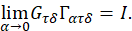
in the strong topology.
Lemma 2.2 [Leiva ~al., 2013] 𝑄 𝜏𝛿 >0 if and only if the linear system (6) is controllable on [𝜏−𝛿,𝜏]. Moreover, given an initial state 𝑦 0 and a final state 𝑧 1 we can find a sequence of controls { 𝑢 𝛼 𝛿 } 0<𝛼≤1 ⊂ 𝐿 2 (𝜏−𝛿,𝜏;𝑈)
𝑢 𝛼 = 𝐺 𝜏𝛿 ∗ (𝛼𝐼+ 𝐺 𝜏𝛿 𝐺 𝜏𝛿 ∗ ) −1 ( 𝑧 1 −𝑇(𝜏) 𝑦 0 ), 𝛼∈(0,1],
such that the solutions 𝑦(𝑡)=𝑦(𝑡,𝜏−𝛿, 𝑦 0 , 𝑢 𝛼 𝛿 ) of the initial value problem
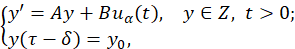
satisfy
lim 𝛼→ 0 + 𝑦(𝜏,𝜏−𝛿, 𝑦 0 , 𝑢 𝛼 )= 𝑧 1 ,
i.e.,
lim 𝛼→ 0 + 𝑦(𝜏)=
lim 𝛼→ 0 + 𝑇(𝛿) 𝑦 0 + 𝜏−𝛿 𝜏 𝑇(𝜏−𝑠)𝐵 𝑢 𝛼 (𝑠) 𝑑𝑠 = 𝑧 1 .
3 Controllability of the Semilinear Equation
In this section we prove the main result of this paper, that is, the approximate controllability of the semilinear impulsive evolution equation given by (1). To this end, for all 𝜙∈𝐶 and 𝑢∈𝐶(0,𝜏;𝑈) the initial value problem
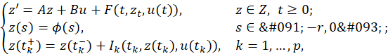
admits only one mild solution 𝑧∈𝑃𝐶(−𝑟,𝜏;𝑍) given by
Now, we are ready to present and prove the main result of this paper, which is the interior approximate controllability of heat equation with delays (1).
Theorem 3.1 Under conditions (H1) and (H2), the semilinear system (1) with impulses and delays is approximately controllable on [0,𝜏].
Proof. Given an initial state 𝜙, a final state 𝑧 1 and 𝜖>0, we want to find a control 𝑢 𝛼 𝛿 ∈ 𝐿 2 (0,𝜏;𝑈) steering the system from 𝜙(0) to an 𝜖-neighborhood of 𝑧 1 at time 𝜏. In other word, there exists control 𝑢 𝛼 𝛿 ∈ 𝐿 2 (0,𝜏; 𝑈) such that corresponding of solutions 𝑧 𝛿,𝛼 of (1) satisfies:
∥ 𝑧 𝛿,𝛼 (𝜏)− 𝑧 1 ∥≤𝜖.
In fact, consider any 𝑢∈ 𝐿 2 (0,𝜏;𝑈) and the corresponding solution 𝑧(𝑡)=𝑧(𝑡,0, 𝑧 0 ,𝑢) of the initial value problem (13). For 𝛼∈(0,1] we define the control 𝑢 ?? 𝛿 ∈ 𝐿 2 (0,𝜏;𝑈) as
𝑢 𝛼 𝛿 (𝑡)= 𝑢(𝑡), if0≤𝑡≤𝜏−𝛿; 𝑢 𝛼 (𝑡), if𝜏−𝛿<𝑡≤𝜏,
where
𝑢 𝛼 (𝑡)=
𝐵 ∗ 𝑇 ∗ (𝜏−𝑡)(𝛼𝐼+ 𝐺 𝜏𝛿 𝐺 𝜏𝛿 ∗ ) −1 ( 𝑧 1 −𝑇(𝛿)𝑧(𝜏−𝛿)),
𝜏−𝛿<𝑡≤𝜏.
Now, assume that 0<𝛿<𝜏− 𝑡 𝑝 . Then the corresponding solution 𝑧 𝛼 𝛿 (𝑡)=𝑧(𝑡,0, 𝑧 0 , 𝑢 𝛼 𝛿 ) of the initial value problem (13) at time 𝜏 can be written as follows:
𝑧 𝛿,𝛼 (𝜏)=
𝑇(𝜏)𝜙(0)+ 0 𝜏 𝑇(𝜏−𝑠)𝐵 𝑢 𝛼 𝛿 (𝑠) 𝑑𝑠
+ 0 𝜏 𝑇(𝜏−𝑠)𝐹(𝑠, 𝑧 𝑠 𝛿,𝛼 , 𝑢 𝛼 𝛿 (𝑠)) 𝑑𝑠
+ 0< 𝑡 𝑘 <𝜏 𝑇(𝜏− 𝑡 𝑘 ) 𝐼 𝑘 ( 𝑧 𝛿,𝛼 ( 𝑡 𝑘 ), 𝑢 𝛼 𝛿 ( 𝑡 𝑘 ))
=𝑇(𝛿) 𝑇(𝜏−𝛿)𝜙(0)+ 0 𝜏−𝛿 𝑇(𝜏−𝛿−𝑠)𝐵 𝑢 𝛼 𝛿 (𝑠) 𝑑𝑠
+ 0 𝜏−𝛿 𝑇(𝜏−𝛿−𝑠)𝐹(𝑠, 𝑧 𝑠 𝛿,𝛼 , 𝑢 𝛼 𝛿 (𝑠)) 𝑑𝑠
+ 0< 𝑡 𝑘 <𝜏−𝛿 𝑇(𝜏−𝛿− 𝑡 𝑘 ) 𝐼 𝑘 ( 𝑧 𝛿,𝛼 ( 𝑡 𝑘 ), 𝑢 𝛼 𝛿 ( 𝑡 𝑘 ))
+ 𝜏−𝛿 𝜏 𝑇(𝜏−𝑠)𝐵 𝑢 𝛼 𝛿 (𝑠) 𝑑𝑠
+ 𝜏−𝛿 𝜏 𝑇(𝜏−𝑠)𝐹(𝑠, 𝑧 𝑠 𝛿,𝛼 ), 𝑢 𝛼 𝛿 (𝑠)) 𝑑𝑠
=𝑇(𝛿)𝑧(𝜏−𝛿)+ 𝜏−𝛿 𝜏 𝑇(𝜏−𝑠)𝐵 𝑢 𝛼 (𝑠) 𝑑𝑠
+ 𝜏−𝛿 𝜏 𝑇(𝜏−𝑠)𝐹(𝑠, 𝑧 𝑠 𝛿,𝛼 , 𝑢 𝛼 (𝑠)) 𝑑𝑠.
Thus,
𝑧 𝛿,𝛼 (𝜏)=𝑇(𝛿)𝑧(𝜏−𝛿)+ 𝜏−𝛿 𝜏 𝑇(𝜏−𝑠)𝐵 𝑢 𝛼 (𝑠) 𝑑𝑠
+ 𝜏−𝛿 𝜏 𝑇(𝜏−𝑠)𝐹(𝑠, 𝑧 𝑠 𝛿,𝛼 , 𝑢 𝛼 (𝑠)) 𝑑𝑠.
The corresponding solution 𝑦 𝛼 𝛿 (𝑡)=𝑦(𝑡,𝜏−𝛿,𝑧(𝜏−𝛿), 𝑢 𝛼 ) of the initial value problem (12) at time 𝜏 is given by:
𝑦 𝛼 𝛿 (𝜏)=𝑇(𝛿)𝑧(𝜏−𝛿)+ 𝜏−𝛿 𝜏 𝑇(𝜏−𝑠)𝐵 𝑢 𝛼 (𝑠) 𝑑𝑠.
Therefore,
∥ 𝑧 𝛿,𝛼 (𝜏)− 𝑦 𝛼 𝛿 (𝜏)∥≤ 𝜏−𝛿 𝜏 ∥𝑇(𝜏−𝑠)∥{𝑎∥ 𝑧 𝛿,𝛼 (𝑠−𝑟)∥+𝑏} 𝑑𝑠.
If we take 0<𝛿<𝑟 and 𝜏−𝛿≤𝑠≤𝜏, then 𝑠−𝑟≤𝜏−𝑟<𝜏−𝛿 and
𝑧 𝛿,𝛼 (𝑠−𝑟)=𝑧(𝑠−𝑟).
Thus, there exists 𝛿 small enough such that 0<𝛿<min{𝑟,𝜏− 𝑡 𝑝 } and
∥ 𝑧 𝛿,𝛼 (𝜏)− 𝑦 𝛿,𝛼 (𝜏)∥ ≤ 𝜏−𝛿 𝜏 ∥𝑇(𝜏−𝑠)∥{𝑎∥𝑧(𝑠−𝑟)∥+𝑏} 𝑑𝑠<𝜖2.
Hence,
∥ 𝑧 𝛿,𝛼 (𝜏)− 𝑧 1 ∥ ≤ 𝜏−𝛿 𝜏 ∥𝑇(𝜏−𝑠)∥{𝑎∥ 𝑧 𝛿,𝛼 (𝑠−𝑟)∥+𝑏} ??
+∥ 𝑦 𝛿,𝛼 (𝜏)− 𝑧 1 ∥= 𝜏−𝛿 𝜏 ∥𝑇(𝜏−𝑠)∥{𝑎∥𝑧(𝑠−𝑟)∥+𝑏} 𝑑𝑠+∥ 𝑦 𝛿,𝛼 (𝜏)− 𝑧 1 ∥<𝜖2+𝜖2<𝜖.
Geometrically, the proof goes as follows:
This completes the proof of the theorem.
4 Applications
As an application, we prove the approximate controllability of the following control system governed by the semilinear wave equation with impulses and delays
where 0< 𝑡 1 < 𝑡 2 < 𝑡 3 <⋯< ?? 𝑝 <𝜏, Ω is a bounded domain in ℝ 𝑛 , the distributed control 𝑢∈ 𝐿 2 ([0,𝜏]; 𝐿 2 (Ω)), 𝜙 0 ∈𝐶(−𝑟,0; 𝐻 2 (Ω)∩ 𝐻 0 1 ), 𝜙 1 ∈𝐶(−𝑟,0; 𝐿 2 (Ω)) and the nonlinear functions 𝑓, 𝐼 𝑘 :[0,𝜏]×ℝ×ℝ×ℝ→ℝ are smooth enough and 𝑓 satisfies (5).
4.1 Abstract Formulation of the Problem
First we choose the space where this problem will be set up as an abstract control system in a Hilbert space. Let 𝑋= 𝐿 2 (Ω)= 𝐿 2 (Ω,ℝ) and consider the linear unbounded operator 𝐴:𝐷(𝐴)⊂𝑋→𝑋 defined by 𝐴𝜙=−Δ𝜙, where

Then the eigenvalues 𝜆 𝑗 of 𝐴 have finite multiplicity 𝛾 𝑗 equal to the dimension of the corresponding eigenspace and 0< 𝜆 1 < 𝜆 2 <⋯< 𝜆 𝑛 →∞. Moreover,
[a)]
1. there exists a complete orthonormal set { 𝜙 𝑗,𝑘 } of eigenvectors of 𝐴;
2. for all 𝑥∈𝐷(𝐴) we have

where <⋅,⋅> is the usual inner product in 𝐿 2 and
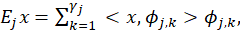
which means the set { 𝐸 𝑗 } 𝑗=1 ∞ is a complete family of orthogonal projections in 𝑋 and 𝑥= 𝑗=1 ∞ 𝐸 𝑗 𝑥, 𝑥∈𝑋;
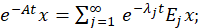
3. −𝐴 generates an analytic semigroup { 𝑒 −𝐴𝑡 } given by
4. the fractional powered spaces 𝑋 𝑟 are given by:
𝑋 𝑟 =𝐷( 𝐴 𝑟 )={𝑥∈𝑋: 𝑛=1 ∞ 𝜆 𝑛 2𝑟 ∥ 𝐸 𝑛 𝑥 ∥ 2 <∞}, 𝑟≥0,
with the norm
∥𝑥 ∥ 𝑟 =∥ 𝐴 𝑟 𝑥∥= 𝑛=1 ∞ 𝜆 𝑛 2𝑟 ∥ 𝐸 𝑛 𝑥 ∥ 2 1/2 ,𝑥∈ 𝑋 𝑟 ,and
Also, for 𝑟≥0 we define 𝑍 𝑟 = 𝑋 𝑟 ×𝑋, which is a Hilbert space endowed with the norm:
𝑦 𝑣 𝑍 𝑟 = ∥𝑦 ∥ 𝑟 2 +∥𝑣 ∥ 2 .
Then, the equations (1) can be written as an abstract second order ordinary differential equations in 𝑍 1/2 as follows
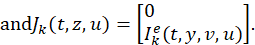
where
𝐼 𝑘 𝑒 :[0,𝜏]× 𝑍 1/2 ×𝑈→ 𝑍 1/2
and
𝑓 𝑒 :[0,𝜏]× 𝐶 0 × 𝐶 1 ×𝑈→ 𝑍 1/2
with 𝐶 0 =𝐶(−𝑟,0; 𝑍 1/2 ) and 𝐶 1 =𝐶(−𝑟,0;𝑍) are defined by
𝐼 𝑘 𝑒 (𝑡,𝑦,𝑣,𝑢)(𝑥)= 𝐼 𝑘 (𝑡,𝑦(𝑥),𝑣(𝑥),𝑢(𝑥)), ∀𝑥∈Ω, 𝑘=1,2,…,𝑝,
𝑓 𝑒 (𝑡, 𝜙 0 , 𝜙 1 ,𝑢)(𝑥)=𝑓(𝑡, 𝜙 0 (−𝑟,𝑥), 𝜙 1 (−𝑟,𝑥),𝑢(𝑥)),
∀𝑥∈Ω, 𝜙 0 𝜙 1 ∈ 𝐶 0 × 𝐶 1 .
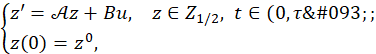
With the change of variables 𝑦′=𝑣, we can write the second order equation (21) as a first order system of ordinary differential equations in the Hilbert space 𝑍 1/2 = 𝑋 1/2 ×𝑋 as follows:
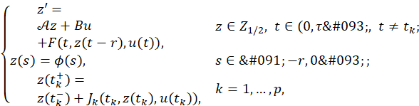
where 𝑢∈ 𝐿 2 ([0,𝜏];𝑈) and 𝐶= 𝐶 0 × 𝐶 1 =𝐶(−𝑟,0; 𝑍 1/2 ),
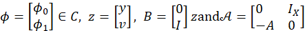
is an unbounded linear operator with domain 𝐷(𝒜)=𝐷(𝐴)×𝐷( 𝐴 1/2 ) and
𝐹(𝑡,𝜙,𝑢)= 0 𝑓 𝑒 (𝑡, 𝜙 0 , 𝜙 1 ,𝑢)
The following result follows from condition (5)
Proposition 4.1 Under the conditions (5) the functions 𝐹 satisfy:

It is well known that the operator 𝒜 generates a strongly continuous group 𝑇(𝑡) 𝑡≥0 in the space 𝑍= 𝑍 1/2 = 𝑋 1/2 ×𝑋 (Chen & Triggiani, 1989). Now, using Lemma 2.1 from Leiva (2003) or Lemma 3.1 from Carrasco & Leiva (2007), one can get the following representation for this group.
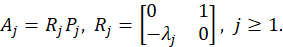
Proposition 4.2 The group 𝑇(𝑡) 𝑡≥0 generated by the operator 𝒜 has the following representation

where 𝑃 𝑗 𝑗≥0 is a complete family of orthogonal projections in the Hilbert space 𝑍 1/2 given by
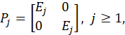
and
4.2 Approximate Controllability
Now, we are ready to formulate and prove the main result of the this section, which is the approximate of the semilinear impulsive wave equation with bounded nonlinear perturbation.
Theorem 4.1 The semilinear wave equation (15) with impulses and delays is approximately controllable on [0,𝜏].
Proof. From Larez et al. (2011), we know that the corresponding linear system without impulses
is controllable on [𝜏−𝛿,𝜏] for all 0<𝛿<𝜏. On the other hand, the hypothesis (H1) and (H2) in Theorem 3.1 are satisfied, and we get the result.
5 Final Remark
This technique can be applied to those systems where the linear part does not generate a compact semigroup, are controllable on any [0,𝛿] for 𝛿>0, and the nonlinear perturbation is bounded. An example of such systems is the following controlled thermoelastic plate equation whose linear part was studied in Larez et al. (2011).
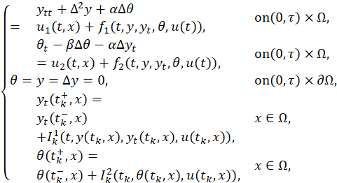
in the space 𝑍= 𝑋 1 ×𝑋×𝑋, where Ω is a bounded domain in ℝ 𝑛 , the distributed controls 𝑢 1 , 𝑢 2 ∈ 𝐿 2 ([0,𝜏]; 𝐿 2 (Ω)) and 𝐼 𝑘 𝑖 , 𝑓 𝑖 are smooth functions with 𝑓 𝑖 ,𝑖=1,2 bounded. Of course, for finite-dimensional control systems, all these results are valid for exact controllability; so from the point of view of applications, we can study real life control systems governed by ordinary differential equations in finite-dimensional spaces, with impulses and delays.

