1 Introduction

There are many works on the existence of bounded solutions without impulses, non-local conditions and delay simultaneously, to mention we have the works done in(^{Leiva, 1999}a, Leiva, 2000, Leiva, 1999b, Leiva & Sivoli, 2003, Leiva & Sequera, 2003, Leiva & Sivoli, 2018, ^{Liu, 2000}, Liu, Naito & Minh, 2006). Recently, in ^{Ayala, Leiva & Tallana (2020}) the existence of solutions for retarded equations with infinite delay, impulses, and non-local conditions has been proved using Karakosta’s fixed point theorem. In ^{Abbas, Al-Arifi, Benchohra & Graef (2020}), the existence of periodic mild solutions of infinite delay evolution equations with non-instantaneous impulses has been studied, by using Poincare map, measure of non-compactness and Darbo fixed point theorem. Compared with these works, in addition we have non-local conditions, and first, we prove the existence of bounded solutions, and under son conditions these bounded solutions are stable, periodic or almost periodic depending on the conditions impose to the linear and non-linear term. Without further ado, in this work we shall study the existence of bounded solutions for the following semi-linear non-autonomous retarded equation with infinite delay, impulses and non-local condition:

z ′ =𝐴(𝑡)𝑧+𝑓(𝑡, 𝑧 𝑡 ), 𝑡>0,𝑡≠ 𝑡 𝑘 , 𝑧(𝑠)+𝑔( 𝑧 𝜏 1 ,⋯, 𝑧 𝜏 𝑞 )(𝑠)=𝜙(𝑠), 𝑠∈(−∞,0)= ℝ − , 𝑧( 𝑡 𝑘 + )=𝑧( 𝑡 𝑘 − )+ 𝐽 𝑘 ( 𝑡 𝑘 ,𝑧( 𝑡 𝑘 )), 𝑘=1,2,⋯,𝑃,

where 𝐴(𝑡) is a continuous 𝑛×𝑛 matrix defined on ℝ, 𝜙∈𝒫𝒲 the space defined as follows

𝒫𝒲={𝜙:(−∞,0]→ ℝ 𝑛 :𝜙 𝑖𝑠 𝑏𝑜𝑢𝑛𝑑𝑒𝑑 𝑎𝑛𝑑 𝑐𝑜𝑛𝑡𝑖𝑛𝑢𝑜𝑢𝑠 𝑒𝑥𝑐𝑒𝑝𝑡 𝑖𝑛 𝑎 𝑓𝑖𝑛𝑖𝑡𝑒 𝑛𝑢𝑚𝑏𝑒𝑟

𝑜𝑓 𝑝𝑜𝑖𝑛𝑡 , 𝑠 𝜙𝑘 ,𝑘=1,2,…,𝑝, 𝑤ℎ𝑒𝑟𝑒 𝑡ℎ𝑒 𝑠𝑖𝑑𝑒 𝑙𝑖𝑚𝑖𝑡𝑠 𝑒𝑥𝑖𝑠𝑡𝑠 𝜙( 𝑠 𝜙𝑘 − ), 𝜙( 𝑠 𝜙𝑘 + )=𝜙( 𝑠 𝜙𝑘 )}

endowed with the norm

∥𝜙 ∥ 𝒫𝒲 =su p 𝑠∈ ℝ − ∥𝜙(𝑠)∥,

where the side limits are defined as follows 𝜙( 𝑠 𝜙𝑘 + )= lim 𝑠→ 𝑠 𝜙𝑘 + 𝜙(𝑠) and 𝜙( 𝑠 𝜙𝑘 − )= lim 𝑠→ 𝑠 𝜙𝑘 − 𝜙(𝑠).

Here, 0< 𝑡 1 < 𝑡 2 <⋯< 𝑡 𝑝 , 0< 𝜏 1 < 𝜏 2 <…< 𝜏 𝑞 , and the functions

𝑔:(𝒫𝒲 ) 𝑞 →𝒫𝒲, 𝐽 𝐾 :ℝ× ℝ 𝑛 → ℝ 𝑛 , 𝑓:ℝ×𝒫𝒲→ ℝ 𝑛

are smooth enough such that the problem (1) admits only one solution 𝑧(𝑡) (see ^{Ayala et al. (2020}) given by

𝑧(𝑡)= 𝑈(𝑡,0)[𝜙(0)−𝑔 𝑧 𝜏 1 ,⋯, 𝑧 𝜏 𝑞 (0)] + 0 𝑡 ‍ 𝑈(𝑡,𝑠)𝑓 𝑠, 𝑧 𝑠 𝑑𝑠+ Σ 0< 𝑡 𝑘 <𝑡 𝑈 𝑡, 𝑡 𝑘 𝐽 𝑘 𝑡 𝑘 ,𝑧 𝑡 𝑘 , 𝑡∈[0,𝜏] 𝑧(𝑠)= 𝜙(𝑠)−𝑔( 𝑧 ?? 1 ,⋯, 𝑧 𝜏 𝑞 )(𝑠), 𝑠∈ ℝ − .

The space (𝒫𝒲 ) 𝑞 is endowed with the usual norm, and 𝑈(𝑡,𝑠)=Φ(𝑡) Φ −1 (𝑠), where Φ(⋅) is the fundamental matrix of the linear system

𝑧 ′ (𝑡)=𝐴(𝑡)𝑧(𝑡),𝑡∈ℝ (1)

i.e.,

Φ ′ (𝑡)=𝐴(𝑡)Φ(𝑡) Φ(0)=𝐼

2 Preliminaries

In this section, we shall choose the space where this problem will be set. To this end, we shall define the following Banach space:

endowed with the norm

∥𝑧 ∥ 𝑏 =su p 𝑡∈ℝ ∥𝑧(𝑡)∥, 𝑧∈𝒫 𝒲 𝑏 .

Now, we shall assume the following hypotheses:

i) 𝑈(𝑡,𝑠)𝑃(𝑠)=𝑃(𝑡)𝑈(𝑡,𝑠), 𝑡,𝑠∈ℝ,

ii) ∥𝑈(𝑡,𝑠)(𝐼−𝑃(𝑠))∥⩽𝑀 𝑒 𝛽(𝑡−𝑠) , 𝑡⩾𝑠,

iii) ∥𝑈(𝑡,𝑠)𝑃(𝑠)∥⩽𝑀 𝑒 𝛽(𝑡−𝑠) , 𝑡⩽𝑠

∥𝑔 𝑧 1 , 𝑧 2 ,… 𝑧 𝑞 ∥ 𝒫𝒲 < ℓ 6 , 𝑧∈𝒫𝒲,

∥𝑔 𝑧 1 ,…, 𝑧 𝑞 −𝑔 𝑤 1 ,⋯, 𝑤 𝑞 ∥ 𝒫𝒲 <𝛾su p 𝑡⩾𝑎 ∥𝑧(𝑡)−𝑤(𝑡) ∥ 𝑞

with

∥𝑧(𝑡)−𝑤(𝑡) ∥ 𝑞 := 𝑖=1 𝑞 ‍ ∥ 𝑧 𝑖 (𝑡)− ?? 𝑖 (𝑡) ∥ ℝ 𝑛 .

Given an interval [𝑎,𝑏] and a ball ℬ 𝛾 (0)⊂𝒫𝒲, there exists a constant 𝒦>0 such that

∥𝑓 𝑡, 𝑧 1 −𝑓 𝑡, 𝑧 2 ∥ ℝ 𝑛 ⩽𝒦|𝑡−𝑠|+∥ 𝑧 1 − 𝑧 2 ∥ 𝒫𝒲 , 𝑧 1 , 𝑧 2 ∈ ℬ 𝛾 (0), 𝑡,𝑠,∈[𝑎,𝑏].

Also, there exists a constant 𝐿 𝑓 >0 such that

∥𝑓(𝑡,0) ∥ ℝ 𝑛 ⩽ 𝐿 𝑓 , 𝑡∈ℝ.

∥ 𝐽 𝐾 𝑡, 𝑧 1 − 𝐽 𝐾 𝑡, 𝑧 2 ∥ ℝ 𝑛 ⩽ 𝑆 𝑘 ∥ 𝑧 1 − 𝑧 2 ∥ ℝ 𝑛 , ∀ 𝑧 1 , 𝑧 2 ∈ ℝ 𝑛 , ∀??∈ℝ;

and

∥ 𝐽 𝐾 (𝑡,0) ∥ ℝ 𝑛 < 𝐿 𝑘 , 𝑘=1,2,⋯,𝑝, 𝑡∈ℝ.

Lemma 1 Under the hypotheses 𝐻1)−𝐻4). A function 𝑧 belonging to 𝒫 𝒲 𝑏 is a solution of (1) if, and only if, 𝑧 is a solution of the following integral equation

𝑧(𝑡)= −∞ ∞ ‍ 𝐺(𝑡,𝑠)𝑓 𝑠, 𝑧 𝑠 𝑑𝑠+ 0< 𝑡 𝑘 ⩽ 𝑡 𝑝 ‍ 𝐺 𝑡, 𝑡 𝑘 𝐽 𝑘 𝑡 𝑘 ,𝑧 𝑡 𝑘 , (2)

𝑧(𝑠)=𝜙(𝑠)−𝑔( 𝑧 𝜏 1 ,⋯, 𝑧 𝜏 𝑞 )(𝑠), 𝑠∈(−∞,0]= ℝ − ,

where 𝐺(𝑡,𝑠) is the Green function defined by

𝐺(𝑡,𝑠)= 𝑈(𝑡,𝑠)(𝐼−𝑃(𝑠)), 𝑡⩾𝑠, −𝑈(𝑡,𝑠)𝑃(𝑠), 𝑡⩽𝑠. (3)

Proof. Suppose that for some 𝜌>0, 𝑧∈ ℬ 𝜌 𝑏 (0)⊂𝒫 𝒲 𝑏 , where ℬ 𝜌 𝑏 (0) is the ball of center zero and radius 𝜌>0 in 𝒫 𝒲 𝑏 , i.e.,

ℬ 𝜌 𝑏 (0)= 𝑧∈𝒫 𝒲 𝑏 :∥𝑧 ∥ 𝑏 <𝜌 .

Let 𝐿 𝜌 be the Lipschitz constant of 𝑓 in ℬ 𝜌 𝑏 (0). On the other hand, we have that

𝑧(𝑡)=𝑈(𝑡,0) 𝜙(0)−𝑔 𝑧 𝜏 1 ,⋯, 𝑧 𝜏 𝑞 (0)

+ 0 𝑡 ‍ 𝑈(𝑡,𝑠)𝑓 𝑠, 𝑧 𝑠 𝑑𝑠+ 0< 𝑡 𝑘 <𝑡 ‍ 𝑈 𝑡, 𝑡 𝑘 𝐽 𝑘 𝑡 𝑘 ,𝑧 𝑡 𝑘

=𝑈(𝑡, 𝑡 0 ){𝑈( 𝑡 0 ,0) 𝜙(0)−𝑔 𝑧 𝜏 1 ,⋯, 𝑧 𝜏 𝑞 (0)

+ 0 𝑡 0 ‍ 𝑈( 𝑡 0 ,𝑠)𝑓 𝑠, 𝑧 𝑠 𝑑𝑠+ 0< 𝑡 𝑘 < 𝑡 0 ‍ 𝑈 𝑡 0 , 𝑡 𝑘 𝐽 𝑘 𝑡 𝑘 ,𝑧 𝑡 𝑘 },

+ 𝑡 0 𝑡 ‍ 𝑈(𝑡,𝑠)𝑓 ??, 𝑧 𝑠 𝑑𝑠+ 𝑡 0 < 𝑡 𝑘 <𝑡 ‍ 𝑈 𝑡, 𝑡 𝑘 𝐽 𝑘 𝑡 𝑘 ,𝑧 𝑡 𝑘 ,

for 𝑡 0 <𝑡. So,

𝑧(𝑡)=𝑈(𝑡, 𝑡 0 )𝑧( 𝑡 0 )+ 𝑡 0 𝑡 ‍ 𝑈(𝑡,𝑠)𝑓 𝑠, 𝑧 𝑠 𝑑𝑠+ 𝑡 0 < 𝑡 𝑘 <𝑡 ‍ 𝑈 𝑡, 𝑡 𝑘 𝐽 𝑘 𝑡 𝑘 ,𝑧 𝑡 𝑘 .

Hence,

(𝐼−𝑃(𝑡))𝑧(𝑡)=(𝐼−𝑃(𝑡))𝑈 𝑡, 𝑡 0 𝑧( 𝑡 0 )+ 𝑡 0 𝑡 ‍ (𝐼−𝑃(𝑡))𝑈(𝑡,𝑠)𝑓 𝑠, 𝑧 𝑠 𝑑𝑠

+ 𝑡 0 < 𝑡 𝑘 <𝑡 ‍ (𝐼−𝑃(𝑡))𝑈 𝑡, 𝑡 𝑘 𝐽 𝑘 𝑡 𝑘 ,𝑧 𝑡 𝑘

=𝑈(𝑡, 𝑡 0 ) 𝐼−𝑃 𝑡 0 𝑧 𝑡 0 + 𝑡 0 𝑡 ‍ 𝑈(𝑡,𝑠)(𝐼−𝑃(𝑠))𝑓 𝑠, 𝑧 𝑠 𝑑𝑠

+ 𝑡 0 < 𝑡 𝑘 <𝑡 ‍ 𝑈 𝑡, 𝑡 𝑘 𝐼−𝑃 𝑡 𝑘 𝐽 𝐾 𝑡 𝑘 ,𝑧 𝑡 𝑘 .

On the other hand,

∥𝑈 𝑡, 𝑡 0 (𝐼−𝑃( 𝑡 0 ))𝑧 𝑡 0 ∥⩽𝑀∥𝑧 𝑡 0 ∥ 𝑒 −𝛽 𝑡− 𝑡 0 , 𝑡 0 ⩽𝑡.

But, ∥𝑧 ∥ 𝑏 <𝜌. Then,

∥𝑈 𝑡, 𝑡 0 𝐼−𝑃 𝑡 0 𝑧 𝑡 0 ∥⩽𝑀𝜌 𝑒 −𝛽 𝑡− 𝑡 0 .

Passing to the limit as 𝑡 0 →−∞, we obtain that

lim 𝑡 0 →−∞ ∥𝑈 𝑡, 𝑡 0 𝐼−𝑃 𝑡 0 𝑧 𝑡 0 ∥=0.

Therefore, we get that

(𝐼−𝑃(𝑡))𝑧(𝑡)= −∞ 𝑡 ‍ 𝑈(𝑡,𝑠)(𝐼−𝑃(𝑠))𝑓(𝑠,𝑧)𝑑𝑠+ 0< 𝑡 𝑘 <𝑡. ‍ 𝑈 𝑡, 𝑡 𝑘 𝐼−𝑃 𝑡 𝑘 𝐽 𝑘 𝑡 𝑘 ,𝑧 𝑡 𝑘 . (4)

Now, let us prove that this improper integral converges.

∥ −∞ 𝑡 ‍ 𝑈(𝑡,𝑠)(𝐼−𝑃(𝑠))𝑓(𝑠, 𝑧 𝑠 )𝑑??∥⩽ −∞ 𝑡 ‍ ∥𝑈(𝑡,𝑠)(𝐼−𝑃(𝑠))𝑓(𝑠, 𝑧 𝑠 )𝑑𝑠

⩽ −∞ 𝑡 ‍ 𝑀 𝑒 −𝛽(𝑡−𝑠) ∥𝑓(𝑠, 𝑧 𝑠 )∥𝑑𝑠

= −∞ 𝑡 ‍ 𝑀 𝑒 −𝛽(𝑡−𝑠) ∥𝑓(𝑠, 𝑧 𝑠 )−𝑓(𝑠,0)+𝑓(𝑠,0)∥𝑑𝑠

⩽ −∞ 𝑡 ‍ 𝑀 𝑒 −𝛽(𝑡−??) ( 𝐿 𝜌 𝜌∥ 𝑧 𝑠 ∥+ 𝐿 𝑓 )𝑑𝑠

= 𝑀( 𝐿 𝜌 𝜌+ 𝐿 𝑓 ) 𝛽 <∞.

Now, we shall suppose that 𝑡 0 >𝑡. Then,

𝑃(𝑡)𝑧(𝑡)=𝑃(𝑡)𝑈(𝑡,0) 𝜙(0)−𝑔(𝑡( 𝑧 𝜏 1 , 𝑧 𝜏 2 ,⋯, 𝑧 𝜏 𝑞 )(0)

+ 0 𝑡 ‍ 𝑃(𝑡)𝑈(𝑡,𝑠)𝑓 𝑠, 𝑧 𝑠 𝑑𝑠+ 0< 𝑡 𝑘 <𝑡 ‍ 𝑃(𝑡)𝑈 𝑡, 𝑡 𝑘 𝐽 𝑘 𝑡 𝑘 ,𝑧 𝑡 𝑘

=𝑃(𝑡)𝑈(𝑡, 𝑡 0 {𝑈 𝑡 0 ,0 𝜙(0)−𝑔 𝑧 𝜏 1 , 𝑧 𝜏 2 ,⋯, 𝑧 𝜏 𝑞 (0)

+ 0 𝑡 0 ‍ 𝑈 𝑡 0 ,𝑠 𝑓 𝑠, 𝑧 𝑠 𝑑𝑠+ 0< 𝑡 𝑘 < 𝑡 0 ‍ 𝑈 𝑡 0 , 𝑡 𝑘 𝐽 𝑘 ( 𝑡 𝑘 ,𝑧( 𝑡 𝑘 ))}

+ 𝑡 0 𝑡 ‍ 𝑈(𝑡,𝑠)𝑃(𝑠)𝑓 𝑠, 𝑧 𝑠 𝑑𝑠+ 0< 𝑡 𝑘 <𝑡 ‍ 𝑈 𝑡, 𝑡 𝑘 𝑃 𝑡 𝑘 𝐽 𝑘 𝑡 𝑘 ,𝑧 𝑡 𝑘

−𝑃(𝑡)𝑈 𝑡, 𝑡 0 0< 𝑡 𝑘 < 𝑡 0 ‍ 𝑈 𝑡 0 , 𝑡 𝑘 𝐽 ?? ( 𝑡 𝑘 ,𝑧( 𝑡 𝑘 ))

=𝑃(𝑡)𝑈 𝑡, 𝑡 0 𝑧 𝑡 0 + 𝑡 0 𝑡 ‍ 𝑈(𝑡,𝑠)𝑃(𝑠)𝑓(𝑠, 𝑧 𝑠 )𝑑𝑠

+ 0< 𝑡 𝑘 <𝑡 ‍ 𝑈 𝑡, 𝑡 𝑘 𝑃 𝑡 𝑘 𝐽( 𝑡 𝑘 ,𝑧( 𝑡 𝑘 ))− 𝑡< 𝑡 𝑘 < 𝑡 0 ‍ 𝑈 𝑡, 𝑡 𝑘 𝑃 𝑡 𝑘 𝐽 𝑘 𝑡 𝑘 ,𝑧 𝑡 𝑘

=𝑈 𝑡, 𝑡 0 𝑃 𝑡 0 𝑧 𝑡 0 + 𝑡 0 𝑡 ‍ 𝑈(𝑡,𝑠)𝑃(𝑠)𝑓 𝑠, 𝑧 𝑠 𝑑𝑠

− 𝑡< 𝑡 𝑘 < 𝑡 0 ‍ 𝑈 𝑡, 𝑡 𝑘 𝑃 𝑡 𝑘 𝐽 𝐾 𝑡 𝑘 ,𝑧 𝑡 𝑘 .

From hypothesis 𝐻1)−𝑖𝑖𝑖), we get that

lim 𝑡 0 →+∞ ∥𝑈 𝑡, 𝑡 0 𝑃 𝑡 0 𝑧 𝑡 0 ∥=0.

Hence,

𝑃(𝑡)𝑧(𝑡)=− 𝑡 ∞ ‍ 𝑈(𝑡,𝑠)𝑃(𝑠)𝑓 𝑠, 𝑧 𝑠 𝑑𝑠− 𝑡< 𝑡 𝑘 ⩽ 𝑡 𝑝 ‍ 𝑈 𝑡, 𝑡 𝑘 𝑃 𝑡 𝑘 𝐽 𝑘 𝑡 𝑘 ,𝑧 𝑡 𝑘 .

Let us prove that this improper integral converges.

∥− 𝑡 ∞ ‍ 𝑈(𝑡,𝑠)𝑃(𝑠)𝑓 𝑠, 𝑧 𝑠 𝑑𝑠∥⩽ 𝑡 ∞ ‍ ∥𝑈(𝑡,𝑠)𝑃(𝑠)𝑓 𝑠, 𝑧 𝑠 ∥𝑑𝑠

⩽ 𝑡 ∞ ‍ 𝑀 𝑒 𝛽(𝑡−𝑠) ∥𝑓 𝑠, 𝑧 𝑠 −𝑓(𝑠,0)+𝑓(𝑠,0)∥𝑑𝑠

⩽ 𝑡 ∞ ‍ 𝑀 𝑒 𝛽(𝑡−𝑠) 𝐿 𝜌 ∥ 𝑧 𝑠 ∥+ 𝐿 𝑓 𝑑𝑠

⩽𝑀 𝐿 𝜌 𝜌+ 𝐿 𝑓 𝑡 ∞ ‍ 𝑒 𝛽(𝑡−𝑠) 𝑑𝑠

=𝑀 𝐿 𝜌 𝜌+ 𝐿 𝑓 𝑒 𝛽(𝑡−𝑠) −𝛽 𝑡 ∞

= 𝑀 𝐿 𝜌 𝜌+ 𝐿 𝑓 𝛽 <∞.

On the other hand,

𝑧(𝑡)=(𝐼−𝑃(𝑡))𝑧(𝑡)+𝑃(𝑡)𝑧(𝑡)

= −∞ ∞ ‍ 𝐺(𝑡,𝑠)𝑓 𝑠, 𝑧 𝑠 𝑑𝑠+ 0< 𝑡 𝑘 ⩽ 𝑡 𝑝 ‍ 𝐺 𝑡, 𝑡 𝑘 𝐽 𝑘 𝑡 𝑘 ,𝑧 𝑡 𝑘 .

Now, suppose that 𝑧 is a solution of the integral equation (2). Then,

𝑧(𝑡)= −∞ 𝑡 ‍ 𝑈(𝑡,𝑠)(𝐼−𝑃(𝑠))𝑓 𝑠, 𝑧 𝑠 𝑑𝑠− 𝑡 ∞ ‍ 𝑈(𝑡,𝑠)𝑃(𝑠)𝑓 𝑠, 𝑧 𝑠 𝑑𝑠

+ 0< 𝑡 𝑘 <𝑡 ‍ 𝑈 𝑡, 𝑡 𝑘 𝐼−𝑃 𝑡 𝑘 𝐽 𝑘 𝑡 𝑘 ,𝑧 𝑡 𝑘 − 𝑡< 𝑡 𝑘 < 𝑡 𝑝 ‍ 𝑈 𝑡, 𝑡 𝑘 𝑃 𝑡 𝑘 𝐽 𝐾 𝑡 𝑘 ,𝑧 𝑡 𝑘 .

Therefore,

− 𝑡< 𝑡 𝑘 < 𝑡 𝑝 ‍ 𝐴(𝑡)𝑈 𝑡, 𝑡 𝑘 𝑃 𝑡 𝑘 𝐽 𝑘 ( 𝑡 𝑘 ,𝑧( 𝑡 𝑘 )).

Hence,

𝑧 ′ (𝑡)=𝐴(𝑡)𝑧(𝑡)+𝑓 𝑡, 𝑧 𝑡 , 𝑡⩾0.

3 Existence of bounded solutions

In this section, we shall prove the existence of bounded solutions for the system (1), and under some conditions, we prove the uniqueness of such a bounded solution. Also, under additional conditions, we prove the stability of these bounded solutions as well.

Theorem 1 Assume the hypotheses 𝐻1)−𝐻4). Let ℬ 𝜌 𝑏 be the ball of center zero and radius 𝜌 in 𝒫𝒲, and 𝐿 𝜌 the Lipschitz constant of 𝑓 in ℬ 2𝜌 . If the following estimate holds

𝜌 1−𝑀 2 𝐿 𝜌 +𝛽𝑆 𝛽 >𝑀 2 𝐿 𝑓 +𝛽 𝐿 𝛽 (5)

where 𝑆= 0< 𝑡 𝑘 <𝑡 ‍ 𝑠 𝑘 and 𝐿 = 𝐾=1 𝑃 ‍ 𝐿 𝑘 , then the system (1) admits one, and only one, bounded solution 𝑧 𝑏 with ∥ 𝑧 𝑏 (𝑡)∥⩽𝜌, 𝑡∈ℝ. Moreover, if additionally we assume that 𝑃(𝑡)≡0 and

5 6 + 3𝑀𝐿𝜌 ?? +3𝑆𝑀<1andℓ⩽𝑆 (6)

this bounded solution is locally stable.

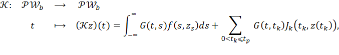
Proof. From Lemma 1, it is enough to prove that the operator

has a fixed point in ℬ 𝜌 𝑏 . For 𝑧∈ ℬ 𝜌 𝑏 , we have the following estimate

∥ 𝒦𝑧 (𝑡) ∥ ℝ 𝑛 ≤ −∞ ∞ ‍ ∥𝐺(𝑡,𝑠)∥∥𝑓 𝑠, 𝑧 𝑠 ∥𝑑𝑠+ 0< 𝑡 𝑘 ⩽ 𝑡 𝑝 ‍ ∥𝐺 𝑡, 𝑡 𝑘 ∥ 𝐽 𝑘 𝑡 𝑘 ,𝑧 𝑡 𝑘 ∥.

From the definition of the Green function, we obtain that

∥𝐺(𝑡,𝑠)∥⩽𝑀 𝑒 −𝛽|𝑡−𝑠| , 𝑡,𝑠∈ℝ.

Therefore,

∥(𝒦𝑧(𝑡)∥⩽ −∞ ∞ ‍ 𝑀 𝑒 −𝛽|𝑡−𝑠| ∥𝑓 𝑠, 𝑧 𝑠 −𝑓(𝑠,0)+𝑓(𝑠,0)∥𝑑𝑠

+ 0< 𝑡 𝑘 < 𝑡 𝑝 ‍ 𝑀 𝑒 −𝛽|𝑡− 𝑡 𝑘 | ∥ 𝐽 𝑘 𝑡 𝑘 ,𝑧 𝑡 𝑘 − 𝐽 𝑘 𝑡 𝑘 ,0 − 𝐽 𝑘 𝑡 𝑘 ,0 ∥

⩽ −∞ ∞ ‍ 𝑒 (𝛽|𝑡−𝑠| 𝐿 𝜌 ∥ 𝑧 𝑠 ∥+ 𝐿 𝑓 𝑑𝑠+ 𝑘=1 𝑃 ‍ 𝑀 𝑆 𝑘 ∥𝑧 𝑡 𝑘 ∥+ 𝐿 𝑘

⩽𝑀 𝐿 𝜌 𝜌+ 𝐿 𝑓 𝑡 ∞ ‍ 𝑒 𝛽(𝑡−𝑠) + −∞ 𝑡 ‍ 𝑒 −𝛽(𝑡−𝑠) +𝑀𝜌 𝑘=1 𝑃 ‍ 𝑠 𝑘 +𝑀 𝑘=1 𝑃 ‍ 𝐿 𝑘

⩽𝑀{ 𝐿 𝜌 𝜌+𝐿𝜌} 1 𝛽 + 1 𝛽 + 𝑀 𝜌 𝑆+𝑀 𝐿

= 2𝑀 𝐿 𝜌 𝜌+ 𝐿 𝑓 𝛽 +𝑀{𝜌𝑆+ 𝐿 }.

From (5), we get that

∥(𝒦𝑧)(𝑡)∥<𝜌∥𝒦𝑧 ∥ 𝑏 <𝜌⇐𝒦(ℬ)⊂ ℬ 𝜌 𝑏 .

∥((𝒦𝑧)(𝑡)−(𝒦 𝑧 )(𝑡)∥∥⩽ −∞ ∞ ‍ 𝑀 𝑒 𝛽|𝑡−𝑠| ∥ 𝑓, 𝑧 𝑠 −𝑓 𝑠, 𝑧 𝑠 ∥ 𝑑𝑠

+ 𝑘=1 𝑃 ‍ 𝑀∥ 𝐽 𝑘 𝑡 𝑘, ,𝑧 𝑡 𝑘 − 𝐽 𝑘 𝑡 𝑘 , 𝑧 𝑡 𝑘 ∥

⩽𝑀 𝐿 𝜌 ∥𝑧− 𝑧 ∥ ∞ ∞ ‍ 𝑒 −𝛽|𝑡−𝑠| 𝑑𝑠

+𝑀 𝑘=1 𝑃 ‍ 𝑆 𝑘 ∥𝑧 𝑡 𝑘 − 𝑧 𝑡 𝑘 ∥

⩽ 2𝑀 𝐿 𝜌 𝛽 ∥𝑧− 𝑧 ∥+𝑀𝑆∥𝑧− 𝑧 ∥

= 2𝑀 𝐿 𝜌 +𝛽𝑀𝑆 𝛽 ∥𝑧− 𝑧 ∥

=𝑀 2 𝐿 𝜌 +𝛽𝑆 𝛽 ∥𝑧− 𝑧 ∥.

From (5), we know that

𝑀 2 𝐿 𝜌 +𝛽𝑆 𝛽 <1,

which implies that 𝒦 is a contraction. Then, applying Banach fixed point Theorem, we get that 𝒦 has a unique fixed point in the ball ℬ 𝜌 𝑏 , i.e., there exists 𝑧 𝑏 ∈ ℬ 𝜌 𝑏 , such that

𝑧 𝑏 =𝒦 𝑧 𝑏 .

Hence,

𝑧 𝑏 (𝑡)= −∞ ∞ ‍ 𝐺(𝑡,𝑠)𝑓(𝑠, 𝑧 𝑠 𝑏 )𝑑𝑠+ 0< 𝑡 𝑘 ⩽ ?? 𝑝 ‍ 𝐺 𝑡, 𝑡 𝑘 𝐽 𝑡 𝑘 , 𝑧 𝑏 𝑡 𝑘 .

To prove that 𝑧 𝑏 (𝑡) is locally stable, we consider any other solution 𝑧(𝑡) of (??) such that 𝑧( 𝑡 0 )− 𝑧 𝑏 ( 𝑡 0 )<𝜌/2. Then ∥𝑧( 𝑡 0 )<2𝜌. As long as 𝑧(𝑡) remains less than 2𝜌, we get the following estimate

𝑡 0 𝑡 ‍ ∥𝑈(𝑡,𝑠)∥∥𝑓 𝑠, 𝑧 𝑠 −𝑓 𝑠, 𝑧 𝑠 𝑏 ∥𝑑𝑠

+ 0< 𝑡 𝑘 <𝑡 ‍ ∥𝑈 𝑡, 𝑡 𝑘 ∥∥ 𝐽 𝐾 𝑡 𝑘 ,𝑧 𝑡 𝑘 − 𝐽 𝑘 𝑡 𝑘 ,𝑧 𝑡 𝑘 ∥.

Since 𝑃(𝑡)≡0, then

∥𝑈(𝑡,𝑠)∥⩽𝑀 𝑒 −𝛽(𝑡−𝑠) , 𝑡⩾𝑠.

Therefore,

+𝑀 𝑡 0 𝑡 ‍ 𝑒 −𝛽(𝑡−𝑠) ∥𝑓 𝑠, 𝑧 𝑠 −𝑓 𝑠, 𝑧 𝑠 𝑏 ∥𝑑

+ 0< 𝑡 𝑘 <𝑡 ‍ 𝑀 𝑒 −𝛽(𝑡− 𝑡 𝑘 ) ∥ 𝐽 𝑘 𝑡 𝑘 ,𝑧 𝑡 𝑘 − 𝐽 𝑘 𝑡 𝑘 , 𝑧 𝑏 𝑡 𝑘 ∥.

Let 𝑡 1 =sup{𝑡> 𝑡 0 :𝑧(𝑡)<2𝜌}. Then either 𝑡 1 =∞ or 𝑧( 𝑡 1 )=2𝜌. Then, from the above estimate one can get that

< 𝜌 2 + 2ℓ 6 +3𝜌 𝑀 𝛽 𝐿 𝜌 +3𝜌𝑀𝑆

< 1 2 + 1 3 + 3𝑀 𝐿 𝜌 𝛽 +3𝑀𝑆 𝜌

= 5 6 + 3𝑀 𝐿 𝜌 𝛽 +3𝑆 𝜌.

Thus,

𝜌< 5 6 + 3𝑀 𝐿 𝜌 𝛽 +3𝑀𝑆 𝜌,

which is a contradiction. Therefore, 𝑡 1 =∞ and 𝑧(𝑡)∈ ℬ 2𝜌 𝑏 , 𝑡⩾ 𝑡 0 . Now, define

∥𝑧− 𝑧 𝑏 ∥ + =su p 𝑡⩾ 𝑡 0 ∥𝑧(𝑡)− 𝑧 𝑏 (𝑡)∥

Then,

∥𝑧− 𝑧 𝑏 ∥ + ⩽∥𝑧 𝑡 0 − 𝑧 𝑏 𝑡 0 ∥+∥𝑔 𝑧 𝜏 1 , … 𝜏 𝑞 −𝑔 𝑧 𝜏 1 ,⋯ 𝑏 , 𝑧 𝜏 𝑞 𝑏 ∥+ 𝐿 𝜌 𝑀 𝛽 ∥𝑧− 𝑧 𝑏 ∥ + +𝑆𝑀∥𝑧− 𝑧 𝑏 ∥ +

⩽∥𝑧 𝑡 0 − 𝑧 𝑏 𝑡 0 ∥+𝛾∥𝑧(⋅)− 𝑧 𝑏 + + 𝑀 𝐿𝜌 𝛽 ∥𝑧− 𝑧 𝑏 ∥ + +𝑆??∥𝑧− 𝑧 𝑏 ∥ +

which implies that

1−Θ− 𝑀 𝐿 𝜌 𝛽 −𝑀𝑆 ∥𝑧− 𝑧 0 ∥⩽∥𝑧( 𝑡 0 )− 𝑧 𝑏 ( 𝑡 0 )∥

By putting Θ=𝛾+ 𝑀 𝐿 𝜌 𝛽 +𝑀𝑆, we obtain that

∥𝑧− 𝑧 1 ?? ∥ + ⩽ 1 1−Θ ∥𝑧( 𝑡 0 )− 𝑧 𝑏 ( 𝑡 0 )∥.

This implies the stability.

To prove the uniqueness of the bounded solution globally, we need the following additional hypothesis:

∥𝑓 𝑡, 𝑧 1 −𝑓 𝑠, 𝑧 2 ∥<𝐿 |𝑡−𝑠|+∥ 𝑧 1 − 𝑧 2 ∥ 𝒫𝒲 ∀𝑡,𝑠,∈ℝ, ∀ 𝑧 1 , 𝑧 2 ∈𝒫𝒲.

Theorem 2 Suppose the hypotheses 𝐻1),𝐻2),𝐻3),𝐻5 hold and

0< 𝑀𝐿 𝛽 +𝑆𝑀< 1 6 .

Then the equation (1) admits one, and only one, bounded solution 𝑧 𝑏 (𝑡) for 𝑡∈ℝ. Moreover, if condition (6) holds, then this bounded solution is globally uniformly stable.

Proof. Let 𝐿>0 be the Lipschitz constant of 𝑓. Then, there exists 𝜌 1 >0 such that

1− 6𝑀𝐿 𝛽 −6𝑀𝑆 𝜌 1 > 𝑀𝐿 𝛽 + 𝐿 𝑀

⇐ 1− 6𝑀𝐿−6𝛽𝑀𝑆 𝛽 𝜌 1 > 𝑀𝐿+𝛽 𝐿 𝑀 𝛽 .

Then, applying Theorem 1, for each 𝜌> 𝜌 1 , we obtain the existence of an unique bounded solution of system (1) in the ball ℬ 𝜌 𝑏 . Hence the problem (1) has one, and only one, globally bounded solution 𝑧 𝑏 . To prove the uniform stability, we assume that 𝑃(𝑡)≡0, consider other solution 𝑧(𝑡) of (1), and the following estimate

∥𝑧− 𝑧 𝑏 ∥ + ⩽ 1 1−Θ ∥𝑧 𝑡 0 − 𝑧 𝑏 𝑡 0 ∥,

where

Θ= 𝛾+ 𝑀𝐿 𝛽 +𝑀𝑆 .

Since Θ does not depend on 𝜌 and 𝑡 0 , the stability is globally uniform.

4 Periodic and Almost periodic solutions

In this section, we shall prove that under some additional conditions, the bounded solutions give by Theorems 1 and 2 are periodic or almost periodic. To this end, in order to prove the periodicity of the bounded solution 𝑧 𝑏 (⋅), we shall assume the following hypotheses:

From the Floquet Theory, there exists a continuous periodic matrix 𝐷(𝑡) and a constant matrix 𝐿 such that for 𝑡∈ℝ

𝐷(𝑡+𝑇)=𝐷(𝑡), 𝑎𝑛𝑑 Φ(𝑡)=𝐷(𝑡) 𝑒 𝐿𝑡 .

From here we get that

Lemma 2 Under the hypotheses 𝐻6)-𝐻7) the unique bounded solution 𝑧 𝑏 (⋅) given in Theorem 1 and Theorem 2 is also T-periodic for 𝑡> 𝑡 𝑝 .

Proof. Let 𝑧 𝑏 be the unique solution of (1) in the ball ℬ 𝜌 𝑏 . Now, we shall prove that 𝑧(𝑡)= 𝑧 𝑏 (𝑡+𝑇 ) 𝑏 is also a solution of (1) in the ball ℬ 𝜌 𝑏 for 𝑡> 𝑡 0 > 𝑡 𝑝 . Observe that

𝑧 𝑠+𝑇 𝑏 (𝑢)= 𝑧 𝑏 (𝑠+𝑢+𝑇)=𝑧(𝑠+𝑢)= 𝑧 𝑢 (𝑠).

Let 𝑡> 𝑡 0 > 𝑡 𝑝 , and consider

𝑧 𝑏 (𝑡)= −∞ ∞ ‍ 𝐺(𝑡,𝑠)𝑓(𝑠, 𝑧 𝑠 𝑏 )𝑑𝑠+ 0< 𝑡 𝑘 ⩽ 𝑡 𝑝 ‍ 𝐺(𝑡, 𝑡 𝑘 )𝐽( 𝑡 𝑘 , 𝑧 𝑏 ( 𝑡 𝑘 ))

= −∞ 𝑡 ‍ 𝑈(𝑡,𝑠)(𝐼−𝑃(𝑠))𝑓(𝑠, 𝑧 𝑠 𝑏 )𝑑𝑠− 𝑡 ∞ ‍ 𝑈(𝑡,𝑠)𝑃(𝑠)𝑓(𝑠, 𝑧 𝑠 𝑏 )𝑑𝑠

+ 0< 𝑡 𝑘 ⩽ 𝑡 𝑝 ‍ 𝑈(𝑡, 𝑡 𝑘 )(𝐼−𝑃( 𝑡 𝑘 )) 𝐽 𝑘 ( 𝑡 𝑘 , 𝑧 𝑏 ( 𝑡 𝑘 ))− 𝑡< 𝑡 𝑘 ⩽ 𝑡 𝑝 ‍ 𝑈(𝑡, 𝑡 𝑘 )𝑃( 𝑡 𝑘 ) 𝐽 𝑘 ( 𝑡 𝑘 , 𝑧 𝑏 ( 𝑡 𝑘 ))

= −∞ 𝑡 0 ‍ 𝑈(𝑡,𝑠)(𝐼−𝑃(𝑠))𝑓(𝑠, 𝑧 𝑠 𝑏 )𝑑𝑠+ 𝑡 0 𝑡 ‍ 𝑈(𝑡,𝑠)(𝐼−𝑃(𝑠))𝑓(𝑠, 𝑧 𝑠 𝑏 )𝑑𝑠

− 𝑡 0 𝑡 ‍ 𝑈(𝑡,𝑠)𝑃(𝑠)𝑓 𝑠, 𝑧 𝑠 𝑑𝑠+ −∞ 𝑡 0 ‍ 𝑈(𝑡,𝑠)𝑃(𝑠)𝑓 𝑠, 𝑧 𝑠 𝑑𝑠

+ 0< 𝑡 𝑘 ⩽ 𝑡 𝑝 ‍ 𝑈 𝑡, 𝑡 𝑘 (𝐼−𝑃( 𝑡 𝑘 )) 𝐽 𝑘 ( 𝑡 𝑘 , 𝑧 𝑏 ( 𝑡 𝑘 ))

= −∞ ∞ ‍ 𝐺(𝑡,𝑠)(𝐼−𝑃(𝑠))𝑓 𝑠, 𝑧 𝑠 𝑏 𝑑𝑠

+ 𝑡 0 𝑡 ‍ 𝐺(𝑡,𝑠)𝑓 𝑠, 𝑧 𝑠 𝑏 𝑑??+ 0< 𝑡 𝑘 ⩽ 𝑡 𝑝 ‍ 𝑈 𝑡, 𝑡 𝑘 (𝐼−𝑃( 𝑡 𝑘 )) 𝐽 𝑘 ( 𝑡 𝑘 , 𝑧 𝑏 ( 𝑡 𝑘 ))

=𝑈(𝑡, 𝑡 0 )[ −∞ ∞ ‍ 𝐺( 𝑡 0 ,𝑠)𝑓(𝑠, 𝑧 𝑠 𝑏 )𝑑𝑠+ 0< 𝑡 𝑘 ⩽ 𝑡 𝑝 ‍ 𝑈 𝑡 0 , 𝑡 𝑘 (𝐼−𝑃( 𝑡 𝑘 )) 𝐽 𝑘 ( 𝑡 𝑘 , 𝑧 𝑏 ( 𝑡 𝑘 ))]

+ 𝑡 0 𝑡 ‍ 𝐺(𝑡,𝑠)𝑓(𝑠, 𝑧 𝑠 𝑏 )𝑑𝑠.

Therefore, for 𝑡> 𝑡 0 > 𝑡 𝑝 , we have that

𝑧 𝑏 (𝑡)=𝑈 𝑡, 𝑡 0 𝑧 𝑏 𝑡 0 + 𝑡 0 𝑡 ‍ 𝐺(𝑡,𝑠)𝑓 𝑠, 𝑧 𝑠 𝑏 𝑑𝑠. (7)

Hence,

=𝑈(𝑡+𝑇, 𝑡 0 ) 𝑧 𝑏 𝑡 0 + 𝑡 0 −𝑇 𝑡 ‍ 𝐺 𝑡+𝑇,𝑠+𝑇 𝑓 𝑠+𝑇, 𝑧 𝑠+𝑇 𝑏 𝑑𝑠

=𝑈 𝑡+𝑇, 𝑡 0 +𝑇 𝑈 𝑡 0 +𝑇, 𝑡 0 𝑧 𝑏 𝑡 0 + 𝑡 0 −𝑇 𝑡 ‍ 𝐺(𝑡,𝑠)𝑓 𝑠, 𝑧 𝑠 𝑑𝑠

=𝑈 𝑡, 𝑡 0 𝑈 𝑡 0 +𝑇, 𝑡 0 𝑧 𝑏 𝑡 0 + 𝑡 0 −𝑇 𝑡 0 ‍ 𝐺(𝑡,𝑠)𝑓 𝑠, 𝑧 𝑠 𝑑𝑠+ 𝑡 0 𝑡 ‍ 𝐺(𝑡,𝑠)𝑓 𝑠, 𝑧 𝑠 𝑑

=𝑈 𝑡, 𝑡 0 𝑈 𝑡 0 +𝑇, 𝑡 0 𝑧 𝑏 𝑡 0 + 𝑡 0 −𝑇 𝑡 0 ‍ 𝐺 𝑡 0 ,𝑠 𝑓 𝑠, 𝑧 𝑠 𝑑𝑠 + 𝑡 0 𝑡 ‍ 𝐺(𝑡,𝑠)𝑓 𝑠, 𝑧 𝑠 𝑑𝑠

=𝑈 𝑡, 𝑡 0 𝑧 0 + 𝑡 0 𝑡 ‍ 𝐺(𝑡,𝑠)𝑓 𝑠, 𝑧 𝑠 𝑑𝑠,

which implies that

𝑧(𝑡)=𝑈(𝑡, 𝑡 0 ) 𝑧 0 + 𝑡 0 𝑡 ‍ 𝐺(𝑡,𝑠)𝑓 𝑠, 𝑧 𝑠 𝑑𝑠,

where

𝑧 0 =𝑈( 𝑡 0 +𝑇, 𝑡 0 ) 𝑧 𝑏 ( 𝑡 0 )+ 𝑡 0 −𝑇 𝑡 0 ‍ 𝐺( 𝑡 0 ,𝑠)𝑓 𝑠, 𝑧 𝑠 𝑑𝑠.

Therefore,

𝑧(𝑡)= 𝑧 𝑏 (𝑡+𝑇)

is a solution of (1) in the ball ℬ 𝜌 𝑏 (0). Hence by the uniqueness of the fixed point in this ball we get that

𝑧 𝑏 (𝑡)= 𝑧 𝑏 (𝑡+𝑇), 𝑡> 𝑡 𝑝

Now, we shall prove that the bounded solution given by Theorem 1 and Theorem 2, under some conditions, is also almost periodic.

Let us assume the following hypotheses:

We recall the following definition and a Theorem from ^{Toka (2017}).

Definition 1. A jointly continuous function 𝑓:ℝ×𝒫𝒲→ ℝ 𝑛 is almost periodic uniformly in 𝜙∈𝑆⊂𝒫𝒲, where 𝑆 is a bounded set, if for any 𝜖>0 there exists ℓ(𝜖)>0 such that for any interval of the form (𝛼,𝛼+ℓ(𝜖)) contains 𝜂 with the property

∥𝑓(𝑡+𝜂,𝜙)−𝑓(𝑡,𝜙)∥<𝜀, ∀𝑡∈ℝ, 𝜙∈𝑆.

Theorem 3. Let 𝑓:ℝ×𝒫𝒲→ ℝ 𝑛 be almost periodic in 𝑡∈ℝ, uniformly in 𝜙∈𝑆⊂𝒫𝒲, where 𝑆 is bounded. Suppose that 𝑓 is globally Lipschitz in 𝜙∈𝒫𝒲. If 𝜁:ℝ→𝒫𝒲 is almost periodic, the function

Γ:ℝ×𝒫𝒲→ ℝ 𝑛 , 𝑑𝑒𝑓𝑖𝑛𝑒𝑑 𝑏𝑦 Γ(𝑡)=𝑓(𝑡,𝜁(𝑡)),

is almost periodic.

Proposition 1. Let 𝑧∈𝒫 𝒲 𝑏 be an almost periodic function. Then, the function

𝜋: ℝ ⟶ 𝒫𝒲 𝑡 ⟼ 𝜋(𝑡)= 𝑧 𝑡 ,

is almost periodic.

Proof. Since 𝑧 is almost periodic, then for every 𝜖>0 there exists ℓ(𝜖)>0 such that any interval (𝛼,𝛼+ℓ(𝜖)) contains 𝜂 such that

∥𝑧(𝑡+𝜂)−𝑧(𝑡)∥<𝜀, ∀𝑡∈ℝ.

Hence

∥𝑧(𝑡+𝜂+𝑠)−𝑧(𝑡+𝑠)∥<𝜀, ∀𝑡,𝑠∈ℝ.

So,

∥𝜋(𝑡+𝜂)−𝜋(𝑡)∥=𝑠𝑢 𝑝 𝑆∈ℝ− ∥ 𝑧 𝑡+𝜂 (𝑠)− 𝑧 𝑡 (𝑠)∥<𝜀, ∀𝑡∈ℝ.

In consequence 𝜋 is almost periodic.

Now, for a function 𝜉∈𝒫 𝒲 𝑏 , we consider the set

𝐻(𝜉)= 𝜉 𝑡 :𝑡∈ℝ ,

the closure in the uniform convergence topology, it is called the Hull of 𝜉, and it is well known (^{Toka, 2017}) that: 𝜉 is almost periodic if, and only if, 𝐻(𝜉) is compact in the uniform convergence topology.

Also, the following statement holds:

For 𝜌>0, the set

𝐴 𝜌 = 𝑧∈ ℬ 𝜌 𝑏 :𝑧 almostperiodic

is closed.

Theorem 4. Under the hypotheses ??8)-𝐻9), the bounded solution 𝑧 𝑏 given by Theorems 1 and 2 is also almost periodic.

Proof. In this case the bounded solution 𝑧 𝑏 can be written as follows

𝑧 𝑏 (𝑡)= −∞ 𝑡 ‍ 𝑒 𝐴(𝑡−𝑠) 𝑓 𝑠, 𝑧 𝑠 𝑑𝑠, 𝑡⩾0

𝑧 𝑏 (𝑠)=𝜙(𝑠), 𝑠∈ ℝ − .

Now, consider the operator 𝒦: 𝐴 𝜌 → ℬ 𝜌 𝑏 given by (7). From proposition 1, we have that

𝜉(𝑡)=𝑓 𝑡, 𝑧 𝑡 , 𝑧∈ 𝐴 𝜌

is almost periodic. On the other hand,

𝒦𝑧 𝑡 = −∞ 𝑡 ‍ 𝑒 𝐴 𝑡−𝑠 𝜉 𝑠 𝑑𝑠.

Next, we will show that 𝐻(𝒦𝑧) is compact in the uniform convergence topology. In fact, consider a sequence {(𝒦𝑧 ) 𝜂 𝑛 } in 𝐻(𝒦𝑧), where (𝒦𝑧 ) 𝜂 𝑛 (𝑡)=(𝒦𝑧)(𝑡+ 𝜂 𝑛 ). Since 𝜉 is almost periodic, there exists a convergent sub-sequence { ℎ 𝜂 𝑛 𝑗 }. Now, we have that

(𝒦𝑧 ) 𝜂 𝑛 𝑗 (𝑡)=(𝒦𝑧) 𝑡+ 𝜂 𝑛 𝑗

= −∞ 𝑡+ 𝜂 𝑛 𝑗 ‍ 𝑒 𝐴 𝑡+ 𝜂 𝑛 𝑗 −𝑠 𝜉 𝑠 𝑑

= −∞ 𝑡 ‍ 𝑒 𝐴(𝑡−𝑠) 𝜉(𝑠+ 𝜂 𝑛 𝑗 )𝑑𝑠.

Then,

∥(𝒦𝑧 ) 𝜂 𝑛 𝑗 (𝑡)−(𝒦 ) 𝜂 𝑛 𝑗 (𝑡)∥⩽ 𝑀 𝛽 ∥ 𝜉 𝜂 𝑛 𝑗 − 𝜉 𝜂 𝑛 𝑖 ∥ 𝑏 .

Thus, {(𝒦𝑧 ) 𝜂 𝑛 𝑗 } is a Cauchy sequence in 𝒫 𝒲 𝑏 , which implies that {(𝒦𝑧 ) 𝜂 𝑛 𝑗 } converges. Hence 𝐻(𝒦𝑧) is compact, and (𝒦𝑧) is almost periodic function. so 𝒦( 𝐴 𝜌 )⊂ 𝐴 𝜌 . Therefore, the only fixed point of 𝒦 on ℬ 𝜌 𝑏 is in 𝐴 𝜌 . Hence, 𝑧 𝑏 (⋅) is almost periodic.

5 Conclusion and Final Remark

In this work, we prove the existence of bounded solutions for retarded equations with infinite delay, impulses, and non-local conditions. This is achieved assuming that the associated linear system has an exponential dichotomy and applying Banach’s fixed point theorem. Then, under certain conditions, we prove that this bounded solution is stable; next, under the additional conditions, we prove that this bounded solution is periodic after the last time impulse 𝑡 𝑝 ; in the same way, under certain conditions, we prove that this bounded solution is almost periodic. We believe that these results can be extended to evolution equations in infinite-dimensional Banach spaces; in fact, this constitutes our next research work in this direction.

Acknowledgment

Many thanks to the anonymous referee for his comments and suggestions to improve the presentation of this work.