


 Spanish (pdf)
 Article in xml format
 Article references
 Send this article by e-mail
 Cited by SciELO
  Similars in
SciELO
Similars in
SciELO 
 Permalink
1 Introduction
In recent years, technological advances have generated a huge variety of new problems and non-linear applications that are commonly seen in major modern engineering applications (Yu & Kaynak, 2009). In this sense, it is well known that the process industries are an integral part of the economic development of a nation and chemical processes use non-linear systems such as distillation columns, boilers, chemical reactors, heat exchangers, among others. These processes are complex, have time delays and different types of non-linearity, higher order, slow dynamic behavior, time delay and external disturbances (Stephanopoulos, 1984). It is not always possible to control them with classic control schemes, such as the feedback control scheme and conventional controllers such as proportional (P), proportional-integral (PI), proportional-integral-derivative (PID), etc.
Thus, general practice of controller design for process control systems requires a mathematical model, however determining an accurate model is almost impossible. Hence, a working model of the plant is obtained using techniques of system identification.
Therefore, to control this type of systems, robust control schemes are required being a concrete approximation to the robust control design the so-called sliding mode control (SMC) method, which constitutes a particular type of control by variable structure. In general, the SMC procedure produces a complex controller, which could contain four or more parameters resulting in a difficult tuning job. Therefore, the use of SMC's traditional procedures presents disadvantages in its application to chemical processes.
There are several papers where successfully designed and applied SMCs for regulation and tracking of systems. Camacho and Smith, (2000) proposed SMC for chemical processes designed from a PID sliding surface and a reduced First Order Plus Delay Time (FOPDT) model of plant with tuning parameters as a function of the characteristic parameters of the FOPDT. Eker (2006) presented a sliding mode control system with a PID sliding surface adopted to control the speed of an electromechanical plant. Herrera et al. (2015), designed and applied a SMC to a Quadrotor, Báez et al. (2018), presented a real implementation of a SMC applied to a cooling tower in an Arduino Mega microcontroller.
In Pérez-Pirela and García-Sandoval (2018) a dynamic model was developed and validated to describe the behavior of a heat exchanger and the proposed SMC for chemical processes was based in this non-linear dynamic model.
The contribution of this paper is that the SMC techniques presented in Camacho and Smith, (2000) and Pérez-Pirela et al. (2018) are simulated for a heat exchanger system to demonstrate applicability of the techniques to practical systems, with integral-differential sliding surface, whose control law is the sum of the switching signal and the equivalent control signal. The results are presented graphically and comparison measures based on time-domain analysis are tabulated. It also presents the potential application in control systems of the representation of radial graphics, because they are an easy way to see how effective the controllers are when the performance of both approaches are compared.
2 Fundamental Sliding-Mode Control
Robustness and systematic design procedures are well-known sliding mode controllers’ advantages (Slotine, 1984). Traditionally, conventional SMC has been designed for systems with relative grade one. If the control input appears on the first derivative of the sliding surface, its relative degree with respect to the control is one. Under these features, the control method is called the first-order SMC. Then, in order to control an output with a relative degree greater than one, it will have to add as many outputs as necessary to display the control input.
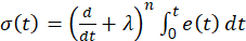
The SMC control law is composed of two parts: the control law of sliding mode and the control law of reach mode. The first is responsible for keeping the dynamic system controlled on a sliding surface, which represents the desired closed-loop behavior. The second control law is designed to reach the desired surface. System trajectories are sensitive to parameter variations and disturbances during trajectory range mode, but are insensitive in slide mode (Sira-Ramírez, 2015). The first step in SMC is the choice of the sliding surface or sliding function that is usually formulated as a linear function of the system states, expressed as a function of the tracking error t ∈ℛ , which is the difference between the measured output and the reference value. In this sense, Slotine (1984) defined an integral-differential sliding surface of order n that applies the complete error of follow-up of the form: (1)
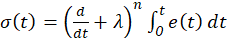
where, 𝑛 is the process order model, and 𝜆 ∈ 𝑅 + is an adjustment parameter. The aim of the control is to ensure that the controlled variable is equal to its reference value at all times, which means that 𝑒 𝑡 and its derivatives must be null. Once the reference value is reached, it indicates that 𝜎 𝑡 reaches a constant value. Keeping 𝜎 𝑡 at this constant value means that 𝑒 𝑡 is zero at all times; that is (2)

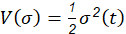
Once the sliding surface is selected, attention must be paid to the design of the control law which drives the controlled variable to its reference value and satisfies equation 2. Thus, the homogeneous differential equation that has a single solution is obtained by fixing 𝑡 . Therefore, the error will come asymptotically to zero with a proper control law that keeps the trajectory on the sliding surface. It is only necessary and sufficient to derive to Equation 1 once, so that the input 𝑢 𝑡 appears. This becomes a first-order stabilization problem based on 𝜎 𝑡 . The direct method of Lyapunov can be used to obtain the control law that maintains 𝜎 𝑡 at zero and a function of Lyapunov candidate is: (3)
with 𝑉 0 =0, 𝑉 𝜎 >0 ∀ 𝜎 𝑒 >0 (Khalil, 2002). A sufficient condition for the stability of the system is: (4)
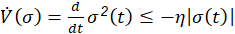
where 𝜂 is a real constant, strictly positive, which determines the speed of convergence of the trajectory to the sliding surface (Slotine, et al.,1991). The inequality of equation 4 ensures that the distance to the sliding surface decreases along all the trajectories and consequently, the system is stable. Therefore, equation 4 is called the attainability condition for the sliding surface. Substituting the sliding surface in equation 4 you get: (5)

Thus, a control input that satisfies the attainability condition can be chosen as: (6)

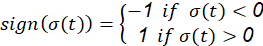
where 𝑓 is the estimate of the equation of state 𝑘, it is the gain of the discontinuous control, which is a strictly positive real constant, with a lower limit that depends on the estimations of the system parameters and external disturbances. The function sign (⋅) denotes the sign function defined as: (7)
The sliding surface design is a powerful tool for improving system performance. It is also possible to shorten the time of reach and thus decrease the effect of the disturbances by increasing the amplitude of the gain of discontinuous control 𝑘 in equation 6.
However, increasing 𝑘 gain has negative effects such as high sensitivity to the dynamics of unmodeled systems, unchattering of amplitude and saturation of the actuator. Therefore, the increase in discontinuous control gain is generally undesirable for physical systems and is not a viable alternative to sliding surface design. A good interchange between the time of reach and the speed of response is obtained by changing the parameters of the sliding surface (Yu & Efe, 2015).
The control input in equation 6 consists of two parts. The first part is a continuous term known as the equivalent control, which is based on the estimated system parameters and compensates for the estimated undesirable dynamics of the system. The second part with the function sign is the law of discontinuous control, which requires an infinite switching by the control signal and the actuator at the intersection of the error trajectory of the state and the sliding surface. Thus, the trajectory is forced to move always towards the sliding surface (Utkin, 1992).
One of the problems generated by the infinity switching or oscillation of the discontinuous control is the chattering effect. This effect produces that in practice the control law cannot be implemented in its natural form, since its direct application will cause the actuators to deteriorate. The main cause of this problem is due to the discontinuous function 𝑠𝑖𝑔𝑛 𝜎(𝑡) which evaluates to the sliding surface. The solution to this problem is to try to make the signal 𝑠𝑖𝑔𝑛 𝜎(𝑡) have a smooth level transition while trying to keep your property. To do this, (Slotine et al., 1991) raises the saturation function as follows: (8)
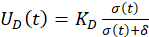
where 𝐾 𝐷 is the setting parameter responsible for the reaching mode, and 𝛿 is a positive constant that helps to reduce the chattering. If 𝛿 is too small, its behavior will resemble the 𝑠𝑖𝑔𝑛 𝜎(𝑡) , so when the controllers are implemented by slider mode, this constant will be chosen so that the control signal prevents the chattering and generates a soft control signal to ensure control objectives.
Methodology
3.1 Experimental Setup
A laboratory-scale heat exchanger was used for the implementation and testing of control strategies based on the sliding mode control method, as shown in figure 1. The heat exchange system was composed of a stainless steel electric heater with a length of 0.29 m, which contains an electrical resistance of 1000 W, the internal and external diameters are d1 =2" y d2 = 1", respectively, and the fluid enters with a temperature T2,i (t) and passes through the heater with a volumetric flow (F) of 2 L/min.
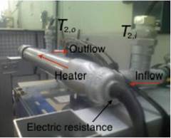
The control objective was to regulate the output temperature of the fluid, 𝑇 2,𝑜 𝑡 , manipulating the power supplied by the electrical resistance, while the initial temperatures ( 𝑇 1,0 𝑧 ∈𝐶 , ?? 2,0 𝑧 ∈𝐶) and inlet temperature, T2,i (t) ϵ C2, are considered as disturbances. Inlet and outlet flow temperatures were measured with J-type thermocouples. The power of the electrical resistance was regulated with a coil relay connected to a PWM device. Fluid flow was controlled by a Asco® Posiflow® proportional solenoid valve model SD8202G086V with a PWM control unit Asco® model 8908A001 using an auxiliary control loop that measures the volumetric flow rate with an FLS® Flow sensor model ULF03.H.0. All signals were read and manipulated with a national Instruments®, Compact Field Point device, operated by the user through a virtual interface developed in LabView, which runs on a desktop PC that communicates with the controller via Ethernet.
3.2 Heat Exchanger Models
Non-Linear Model
Based on a distributed parameter model for the heat exchanger described in the previous section, (Pérez-Pirela et al., 2018) developed a simplified mathematical model for this system, which describes the dynamic behavior of the temperature at the output (𝑇2,𝑜), by means of an ordinary differential equation of second order with delay in the input (u), and the disturbances (𝑇2,𝑖 y 𝐹): (9)
where (10)
and 𝑝 𝑡 is an auxiliary variable whose dynamic is (11)
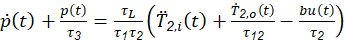
with initial conditions 𝑇 2,𝑜 0 = 𝑇 0 y 𝑝 0 =0 . Here, 𝜏 𝑖 = 𝐴 𝑖 𝜌 𝑖 𝑐 𝑣,𝑖 /ℎ𝑝 , for 𝑖=1,2; are the characteristic times of heat transport for each material (resistance 𝑖=1 y fluid 𝑖=2 ), 𝜏 12 −1 = 𝜏 1 −1 + 𝜏 2 −1 is the overall characteristic time, 𝜏 𝐿 =𝐿 𝐴 2 /𝐹 is the time of fluid residency within the exchanger, 𝑏=1/ 𝐴 1 𝐿 𝜌 1 𝑐 𝑣,1 and 𝑢( 𝑡 ) = 𝑉 2 ( 𝑡 ) /𝑅 is the control variable (for more details consult (Pérez-Pirela et al., 2018). By observing equation 9, it is clear that the relative degree between the 𝑢 and the 𝑇 2,𝑜 output is two.
First Order Plus Dead Time (FOPDT) Model
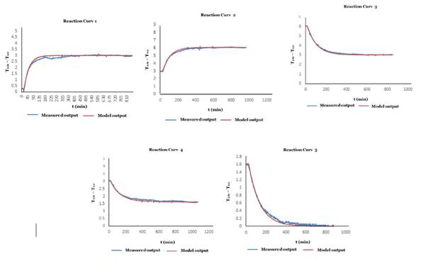
The reaction curve of the process, figure 2, is a commonly used method for the identification of dynamic models (Smith & Corripio, 1997). This method is simple to perform and provides suitable models for many applications; thus, the first-order model with delay is used to approximate the model of the heat exchanger system. For this purpose, the curve is obtained by introducing a series of step changes in the output of the controller through the power of the electrical resistance as shown in table 1 and recording the output of the transmitter with the output temperature of the fluid.
In this way, when performing the step tests, the following reaction curves are obtained for the system, it is shown in figure 2:
In this way it is able to provide a reduced suitable model for the application of the heat exchanger. From the process curve shown in figure 2, and the procedure presented in (Smith & Corripio,1997); the numerical values of the terms of the FOPDT model given in equation 12 are obtained:
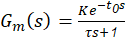
where 𝐾 is the static gain, 𝜏 is the time constant and 𝑡 0 is the delay time. Using the input/output data for the system, the average coefficients of the plant are =6 , 𝜏=101 y 𝑡 0 =23.
The dynamic behavior of the non-linear model and the reduced order model are shown in figure 3; it can be seen an acceptable deviation in both models.

3.3 Sliding Mode Control Algorithms
The results are presented to demonstrate the operation of two selected SMC techniques which mainly characterize the classic SMC for the purpose of regulating error 𝑒( 𝑡 ) = 𝑇 2,𝑜 − 𝑇 2,𝑟 . Controller parameters are tuned during experiments, avoiding complicated calculations that can cause large chattering that is dangerous to the actuator.
Technique I: This technique is presented to regulate chemical processes by Camacho y Smith (2000), applying a reduced FODPT model; and the control signal is the sum of the switching signal and the equivalent control signal.
Technique II: This technique was proposed by (Pérez-Pirela et al., 2018), where conventional SMC techniques applied to an experimental non-linear heat exchanger model are designed, validated and compared. The control law is the sum of the switching signal and the equivalent control signal.
In both techniques a sliding surface is used based on the integral of the error, for a heat exchange system, the sliding surface related to 𝑛=2 is the one shown below (13)
The control signal is the sum of the switching signal and the equivalent control signal.
Simulations were performed for the heat exchanger coupled with each controller. The initial conditions of the system, Begin with the heat exchanger being in is in permanent mode at a temperature of thermal equilibrium of 25 ° 𝐶, with a volumetric flow of 2 𝐿/𝑚𝑖𝑛 , an inlet temperature, 𝑇2,𝑖; variable as load disturbance. At 𝑡=0 𝑚𝑖𝑛 the controller started with a reference temperature of 27 °𝐶 , then at 𝑡=50 𝑚𝑖𝑛 the reference temperature was changed to29 °𝐶, then to 𝑡=75 𝑚𝑖𝑛 to decrease the reference temperature to 28 ° t , thus it is intended to measure the characteristics of tracking to a system reference. Subsequently, the volumetric flow was decreased to 1.3 𝐿/𝑚𝑖𝑛 and the previously commented tests were performed again, in order to observe the system behavior before the variation in one of its nominal parameters.
The performance of the techniques was evaluated with the following performance indices:
The integral of the absolute error (IAE) = ∫|𝑒(𝑡)|𝑑𝑡
The integral of the control input Absolute (IACI) = ∫|𝑢 𝑡 |𝑑𝑡.
Results and Discussion
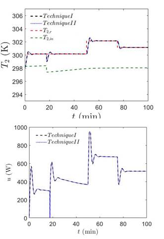
The controllers of the techniques were implemented in the MATLAB environment and the sampling time was selected to be 100 s. To test the system's regulatory properties, the reference temperature changes mentioned in subsection 2.3 were applied and the responses are shown in figure 4. This figure shows, that both techniques have a very similar performance, so it was also compared to the performance indices presented in table 2. These results show that the system with the technique II sliding mode controller has better performance than the system with technique I.
The controllers of the techniques were implemented in the MATLAB environment and the sampling time was selected to be 100 s. To test the system's regulatory properties, the reference temperature changes mentioned in subsection 2.3 were applied and the responses are shown in figure 4. This figure shows, that both techniques have a very similar performance, so it was also compared to the performance indices presented in table 2. These results show that the system with the technique II sliding mode controller has better performance than the system with technique I.
Table 2: Performance Index results to changes in the reference.
| Techniques SMC | IAE | IACI |
|---|---|---|
| I | 619.29 | 4.8905× 10⁴ |
| II | 611.05 | 4.8854× 10⁴ |
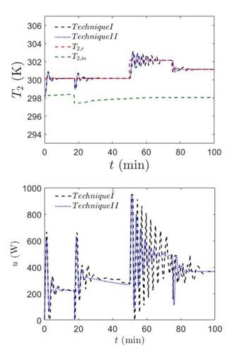
To test the robustness of the system in the face of parameter variation, the volumetric flow was decreased to 1.3 L/min and the results are shown in figure 5. The performance of the techniques was also compared to performance indices and presented in table 3. The system with conventional SMC oscillates during the recovery of the disturbance, showing that technique II again has better performance than technique I.
Table 3: Performance Index results to parameter variation.
| Techniques SMC | IAE | IACI |
| I | 968.03 | 3.6030 × 10⁴ |
| II | 694.16 | 3.5860× 10⁴ |
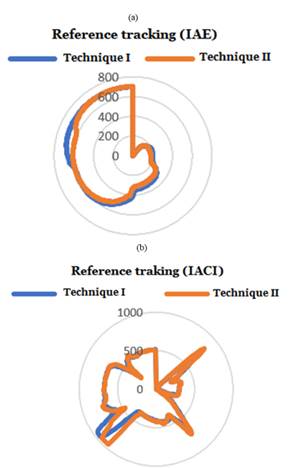
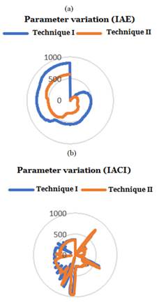
In this work, we also wanted to show the results in the representation of radial charts, because radial charts are the most effective when you are comparing target vs achieved performance to a standard or a group's performance. Figure 6 shows the controllers’ performance to the reference temperature changes for both techniques; thus, they can be easily compared along their own axis, and the global similarities are evident by the size and shape of the polygons that are generated. Similarly, figure 7 shows the performance of the controllers by decreasing the flow from 2 L/min to 1.3 L/min, and overall differences are apparent by the size and shape of the polygons.
5 Conclusion
In this study, two conventional sliding mode control techniques selected for an experimental heat exchanger system have been evaluated to investigate the applicability of the proposed techniques. A first-rate model with delay approaches its use in experiments, as most real systems can be represented by a reduced first-order model with delay. The step response, the control signal and the variations of the switching signal, error versus failure derived from the error were obtained to compare the performances of the techniques. During the experiments, the parameters were tuned manually, as the presence of chattering can cause a detrimental effect on the system components.
According to the results and analysis in the time domain tabulated in table 2 and table 3, it is clear that the techniques presented in (Pérez-Pirela et al., 2018), have produced better results than the technique presented in (Camacho et al., 2000). Both techniques have less chattering in the control signal than can be acceptable for the actual systems. Since the tracking error converges exponentially to zero under uncertainties, the SMC techniques presented in (Camacho et al., 2000) and (Pérez Pirela et al., 2018) can be candidates for their use in industrial applications as an alternative to the PID controller commonly used. In addition, the first-order slider-mode control algorithm has always systematic solution. So, it is easy to understand and apply to real systems.

