


 Español (pdf)
 Articulo en XML
 Referencias del artículo
 Enviar articulo por email
 Citado por SciELO
  Similares en
SciELO
Similares en
SciELO 
 Permalink
Introduction
Background
The lack of analytical methods in the field of industrial electrical trunking systems , for determining corrosion effects on metal coatings, makes optimal coating selection difficult, since current methods don´t use any scientific methodology that considers the different environmental parameters that take part in the corrosion of the coating. In this regard, the coating selected in a heuristic way, usually does not meet the requirements regarding corrosion resistance; thus, the expected life of the trunking system could be drastically reduced or, on the contrary, could be unnecessarily overqualified.
In order to minimize these problems, it is necessary to provide a methodology for calculating atmospheric corrosion, considering all parameters that take part in this process including meteorological factors (e.g. relative humidity, number of rainy days, temperature, among others) and pollutants (mainly, chlorine and sulphur ions).
Manufacturers’ recommendations
Overall, the technical literature from manufacturers generally includes a categorization of the type of environments and the recommended coating for each, as it is shown in table 1 (Chenoll Mora, 2005). However, no manufacturer provides any scientific method to accurately determine the atmospheric corrosion of the metal, considering the meteorological and pollutant parameters of the location.
Logarithmic general expression
The current methods of quantitative calculation for atmospheric corrosion are generally based on two steps:
Calculation of corrosion after one year (first year of exposure)
Calculation of the corrosion for any period of time (beyond one year of exposure)
As shown in previous studies (CEN, European Committee for Standardization, 2012; Feliu Batlle, Morcillo, & Feliu, 1993a; González Fernández & Consejo Superior de Investigaciones Científicas (CSIC), 1984; Pourbaix, 1982b), the corrosion in most of the cases, is estimated by means of bi-logarithmic expressions of the type:
where,
The non-linearity of corrosion function, 𝐶 𝑡 , is a key element in understanding the corrosion process over time. In fact, this non-linear model positively modifies the estimated lifetime of the installation and consequently, its economic impact.
Likewise, it is well known that the corrosion process is, in most cases, stabilized for 𝑡>20 having a linear behaviour. Therefore, the corrosion function (𝐶) can be obtained as follows (CEN, European Committee for Standardization, 2012; Morcillo, 1998; Panchenko & Marshakov, 2016):

Corrosion during the first year of exposure (A)
Following a literature review on different methodologies, ten studies were selected in order to determine the best fitting model to actual corrosion values. table 2 shows the different variables and parameters considered on those techniques.
Method 1: Applicable in atmospheres exempt from contamination (Chico, De La Fuente, Vega, & Morcillo, 2010; Feliu & Morcillo, 1980. 2013; Morcillo & Feliu, 1987).3
Method 2: Applicable in atmospheres exempt from contamination. This method is based on the same study from which Method 1 comes from. (4)
Table 1: Summary of coatings recommended by the main cable tray manufacturers (Chenoll Mora, 2005).
| Corrosivity category ISO 9223 | Environments defined by manufacturers | Type of coatings | ||||||||
| Electro-plated (ISO 2081) | Bi-chromate electro-plated (ISO 2081) | Pre-Galv. (EN 10346) | Hot-Dip Galv. (ISO 1461) | Stainless steel AISI 304 | Stainless steel AISI 316 | Epoxy-polyester | Rilsan® (PA) Levasint® (PE) | Aluminium | PVC | Galv. + epoxy |
| C1: Very low | In-door (normal environment) | S | O | S | O | |||||
| Chemical industry / Aseptic | I | S | I | S | I | |||||
| Any C1 environment | S | O | S | O | ||||||
| C2: Low | Out-door (normal environment) | I | P (1) | S | O | P | O | P | ||
| Food industry | I | S | O | I | S Levasint® | S | I | |||
| Abrasive environment | P | S | O | S | S Levasint® | O | P | S | ||
| Any C2 environment | I | P (1) | S | O | P | O | P | O | ||
| C3: Medium | Alkaline environment | I | P | S | P | S | P | |||
| Hydrocarbons | I | P | S | NIA | ||||||
| Organic acids | I | P | S | NIA | ||||||
| Out-door moderated severity | I | P | S | NIA | ||||||
| Any C3 environment | NIA | I | S | O | NIA | O | ||||
| C4: High | Acid environment | I | P | S | P | S | I | S | P | |
| Seashore | I | P | I | S | NIA | |||||
| Mineral acids | I | P | S | NIA | ||||||
| Caustic soda | I | P | S | NIA | ||||||
| Indoor aggressive environment | I | P | S | NIA | ||||||
| Any C4 environment | NIA | I | S | O | NIA | O | ||||
| C5-I: Very high (industrial) | Halogen environment | I | S | P | S | |||||
| Chlorine | I | P | S | NIA | ||||||
| Industrial environment (humid - sulphurous) | NIA | I | P | S | NIA | Levasint® | S | NIA | S | |
| Any C5-I environment | NIA | I | S | NIA | S | |||||
| C5-M: Very high (marine) | Marine environment, aggressive, sulphurous | I | P | S | I | S | P | |||
| Any C5-M environment | NIA | I | S | NIA | S |
Note: (S) Suitable; (I) Inadequate; (O) Overqualified; (P) Possible (2); NIA: No Information Available (3)
The electroplated bi-chromate and the Pre-Galvanized finishes can be used in normal outdoor environments, understood as such, by dry environments or with very low humidity levels. If it is a clean environment (low pollution), but with the possibility of reaching high relative humidity, this type of environment would change to a higher classification range, as C3 or C4.
It is possible to use the coating, although it is not the optimal option. In these cases, further important parameters of the installation should be studied in more depth: humidity, temperature, pollution, temperature gradients, atmospheric conditions, among others, to ensure that the coating can be used.
(3) The manufacturer who defines this type of environment, does not manufacture this type of finish, so no information is available in that respect.
(4) Sources: Thorsman, Permisa, Industrias Eléctricas Pinazo, Porime, Latina Canale SRL, NLC Sistema Metallici, Aemsa, Apiem
Table 2: Variables and parameters used in the methods to estimate annual corrosion (A).
| Variable / Parameter | Description / Value | Units |
|---|---|---|
| Ax | Corrosion at first year of exposure calculated with method x | Microns (µm) |
| RH | Average annual relative humidity | % |
| T | Average annual temperature | ºC |
| L | Number of rainy days per year | Days |
| W | Wetness time estimated, as the number of hours in one year during which RH ( 80% and T > 0°C simultaneously (ISO, International Organization for Standardization, 2012) | Hours |
| M | Corrosion module for 1000 h of wetness of the metal surface in a pure atmosphere (free of contaminants); for the case of zinc it corresponds to 0.4 (m | µm |
| tw | Wetness time | Hours/1000 |
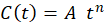
| ft | Coefficient of corrosion inhibition with the annual wetness time (t) | Constant |
| ⍺ | Influence of SO2 contamination | Constant |
| ß | Influence of Cl- contamination | Constant |
| fc | Stimulating coefficient of corrosion due to contaminants in the air | Constant |
| Cl-: | Average annual concentration of chlorides | mg·(m-2·d-1) |
| S | Average annual concentration of sulphur dioxide (SO2) | mg·(m-2·d-1) |
| S* | Average annual concentration of SO2 + Cl- | mg·(m-2·d-1) |
| Pd | Annual average SO2 deposition | mg·(m-2·d-1) |
| fZn | 0.038·(T - 10) when T <= 10 °C; otherwise, -0.071·(T - 10) | ºC |
| Sd | Annual average Cl- deposition | mg·(m-2·d-1) |
| D | Day | - |
Method 3: Applicable in atmospheres exempt from contamination (Costa, Mercer, Institute of Materials of London, European Federation of corrosion, & Sociedad Española de Química Industrial, 1993). See(5)
Method 4: Applicable in any type of atmosphere (Morcillo & Feliu, 1993). See(6)
Where fc is calculated through the following expression: See(7)

Coefficient ft and parameters 𝛼 and 𝛽, can be obtained by the following graphs in Figures 1-3.
Method 5: Applicable in contaminated atmospheres (Morcillo, 1998; Morcillo & Feliu, 1993). See(8)
Method 6: Applicable in any type of atmosphere (Almeida, Rosales, Uruchurtu, Marroco, & Morcillo, 1999). See(9)
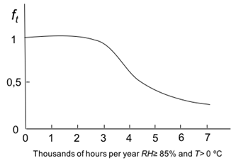
Figure 1: Variation of f t , versus wetness time. Source: own illustration based on reference (Morcillo & Feliu, 1993).
Method 7: Applicable in contaminated atmospheres. This method is part of the same study as that referenced in Method 10: See (10)
Method 8: Applicable in any type of atmosphere (ISO, International Organization for Standardization, 2012): See (11)
Method 9: Applicable in any type of atmosphere (Haagenrud, Henriksen, & Gram, 1985): See (12)
Method 10: Applicable in contaminated atmospheres (Benarie & Lipfert, 1986; Feliu Batlle et al., 1993a; Feliu Batlle, Morcillo, & Feliu, 1993b; Morcillo, 1998): See (13)
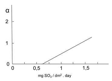
Figure 2: Variation of ( versus mean values of SO2. Source: own illustration based on reference (Morcillo & Feliu, 1993)
Figure 3: Variation of ( versus mean values of chlorides. Source: own illustration based on reference (Morcillo & Feliu, 1993).
Estimation of the parameter n
Several examples have been used to determine the parameter n (equations 1 & 2), of which the following were selected:
It is commonly accepted (CEN, European Committee for Standardization, 2012; Chico et al., 2010; Hernández, Miranda, & Domínguez, 2002) that for the case of zinc, n-parameter is usually in the range of 0.8 to 1, although this range depends on the type of environment of the installation.
For his part, M. Pourbaix (Pourbaix, 1982a) facilitates reference values, which are showed in table 3.
M. Morcillo (Morcillo, 1998) makes the analysis for exposures over 10 years (Table 4), based on actual field trials within the ISO CORRAG program (Dean & Reiser, 2002; Knotkova, Boschek, & Kreislova, 1995; Knotkova, Dean, & Kreislova, 2010; Panchenko, Marshakov, Igonin, Kovtanyuk, & Nikolaeva, 2014).
Table 3: Possible values of n-parameter for different types of atmospheres (Pourbaix, 1982a).
| Rural atmosphere | Urban-Industrial atmosphere | Marine atmosphere |
|---|---|---|
| 0.65 | 0.9 | 0.9 |
Table 4: n ranges obtained in long-term exposures (10-20 years) (Morcillo, 1998).
| Rural-Urban atmosphere away from the sea | Industrial atmospheres away from the sea | Marine atmosphere |
|---|---|---|
| 0.8 - 1 | 0.9 - 1 | 0.7 - 0.9 |
The standard EN ISO 9224 (CEN, European Committee for Standardization, 2012), gives two values for n: B1 and B2 (table 5). For general applications, n will take the value of B1. In those cases, where it is important to estimate a more conservative corrosion attack limit after long exposures, the value of B should be increased to consider the uncertainties of the values of B1. Value B2 includes these uncertainties. Therefore, the use of B1 or B2 as the parameter n, will clearly depend on the degree of accuracy that is intended for the calculation
Table 5: n-parameter values for predicting and estimating zinc corrosion attack according to EN ISO 9224 (CEN, European Committee for Standardization, 2012).
| B1 | B2 |
| 0.813 | 0.873 |
Regarding the previous standard, it is also advisable to use a value of 1 for n, for in the cases of installations in environments with a high content of sulphur dioxide, it is assumed that the corrosion of zinc is almost linear.
From this analysis, the designer must choose the most appropriate value of n, considering these general recommendations:
As a general value, the one established by EN ISO 9224 (CEN, European Committee for Standardization, 2012), can be taken.
For t > 20 years, values between 0.9 and 1 should be chosen, because the zinc corrosion ratio becomes linear from this exposition time (CEN, European Committee for Standardization, 2012).
For environments with very high concentrations of sulphur dioxide (P3), values between 0.9 and 1 should be used (CEN, European Committee for Standardization, 2012).
For exposures in rural environments with very low pollution rates and for exposures around 10 years, lower values should be used for n, according to the previous tables, but not below 0.65.
Finally, it is advisable to review the information provided in the aforementioned ISO CORRAG program, which is used in many research studies in the field of corrosion (Dean & Reiser, 2002; Knotkova et al., 1995. 2010; Panchenko et al., 2014).
Methodology
Comparative analysis of annual corrosion, between current theoretical methods and actual field tests
This section aimed to verify the adequacy of the current methods used to determine corrosion prediction for the first year of exposure, versus actual corrosion values measured in field tests. In this way, the parameters corresponding to 15 different test stations, each having distinct atmospheric natures, were used: 13 from the Iberian Peninsula, 1 in France and 1 in Finland. From these parameters, the corrosion for the first year of exposure for each of the 10 above-mentioned methods (A x ) was calculated and compared with the actual values measured at such test stations.
The results of the analyses are shown in tables 6-table 8, including the following information:
Meteorological and environmental parameters (RH, T, L, W, Cl - , S).
Results of calculated corrosion values (A x ) for each of the methods specified.
Actual corrosion values (Morcillo & Feliu, 1993; Panchenko & Marshakov, 2016).
The difference between theoretical predicted values and the actual results for each of the methods. Here, methods with the least differences are highlighted.
The average of the differences of each method and its standard deviation, as fundamental data, to decide the method that best fits all the analyzed scenarios.
The meteorological and environmental records of these stations were extracted from the data of the actual corrosion value field tests (Morcillo & Feliu, 1993; Panchenko & Marshakov, 2016). There are also alternative sources to get this parameters like national meteorological institutes, web sites (“Weather and Climate: Average monthly Rainfall, Sunshine, Temperatures, Humidity, Wind Speed,” n.d.; “World climate data - Temperature, Weather and rainfall,” n.d.), etc.
From the results, the following conclusions were taken into account for designing the proposed methodology:
Method 1, is the procedure that best matches the actual values of corrosion: lowest average of differences (0.46 μm) and standard deviation (0.53 μm). This method is only applicable to rural atmospheres (classes C1 to C3 according to ISO 9223 (ISO, International Organization for Standardization, 2012).
Method 4, is the one that best fits the actual test values for contaminated atmospheres (classes C4 to CX according to ISO 9223 (ISO, International Organization for Standardization, 2012): lowest average of differences (1.19 μm) and standard deviation (1.78 μm). This method could be used also for rural atmospheres.
The accuracy of the adjustment against actual values of the methods for rural environments is quite good, with not one average deviation exceeding 0.8 microns, therefore, it could be said that any of these methods could be used.
Methods 9 and 10 were discarded, since they predicted theoretical corrosion values very distant to the actual results.
Flow-chart
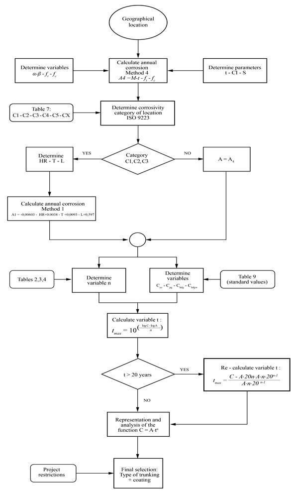
Figure 4 illustrates the methodology proposed for the optimal selection of a zinc-coated cable trunking system, against atmospheric corrosion.
Predicted corrosion values for the first year of exposure versus actual test stations values (Part I).
| Test station location | Alicante (Spain, 30 m from sea) | Alicante (Spain, 100 m from sea) | El Escorial (Madrid-Spain, 1032 m from sea) | Bilbao (Spain, 6 m from sea) | Barcelona (Spain, 13 m from sea) | Cabo Negro (Javea -Spain, 12 m from sea) | Zaragoza (Spain, 320 m from sea) | Avilés (Spain, 139 m from sea) | |||||||||
|---|---|---|---|---|---|---|---|---|---|---|---|---|---|---|---|---|---|
| Variable | Value | Value | Value | Value | Value | Value | Value | Value | |||||||||
| RH (%) | 65 | 65 | 62 | 82 | 70 | 65 | 61 | 78 | |||||||||
| T (ºC) | 18.75 | 18.75 | 13.75 | 13.75 | 16.25 | 13.75 | 13.75 | 13.75 | |||||||||
| L (days) | 91 | 91 | 101 | 153 | 100 | 91 | 94 | 193 | |||||||||
| W (hours) | 4300 | 4300 | 3900 | 3000 | 3200 | 4300 | 2100 | 3700 | |||||||||
| M (0.4 µm) | 0.4 | 0.4 | 0.4 | 0.4 | 0.4 | 0.4 | 0.4 | 0.4 | |||||||||
| tw (thousand hours per year) | 4.3 | 4.3 | 3.9 | 3 | 3.2 | 4.3 | 2.1 | 3.7 | |||||||||
| ft | 0.5 | 0.5 | 0.65 | 0.9 | 0.95 | 0.5 | 1 | 0.7 | |||||||||
| ⍺ | 1.2 | 0 | 0 | 0.5 | 0.4 | 0 | 0.2 | 0 | |||||||||
| ß | 4.4 | 0 | 0 | 1.8 | 1.3 | 4 | 0 | 0 | |||||||||
| fc (1+⍺+ß) | 6.6 | 1 | 1 | 3.3 | 2.7 | 5 | 1.2 | 1 | |||||||||
| Cl- (mg Cl- / m2.d) | 166 | 25 | 0 | 67 | 45 | 118 | 0 | 0 | |||||||||
| S (mg SO2 / m2.d) | 155 | 21 | 15 | 101 | 86 | 30 | 57 | 48 | |||||||||
| S* (mg / m2.d) | 321 | 46 | 15 | 168 | 131 | 148 | 57 | 48 | |||||||||
| Pd (mg / m2.d) | 155 | 21 | 15 | 101 | 86 | 30 | 57 | 48 | |||||||||
| Sd (mg / m2.d) | 166 | 25 | 0 | 67 | 45 | 118 | 0 | 0 | |||||||||
| fZn | -0.621 | -0.621 | -0.266 | -0.266 | -0.444 | -0.266 | -0.266 | -0.266 | |||||||||
| "A" Calculation method | Value | Diff. | Value | Diff. | Value | Diff. | Value | Diff. | Value | Diff. | Value | Diff. | Value | Diff. | Value | Diff. | |
| A1 (µm) - 1: Rural | - | - | 1.16 | 0.44 | 1.26 | 1.34 | - | - | - | - | - | - | 1.20 | -0.10 | 2.06 | -0.56 | |
| A2 (µm) - 2: Rural | - | - | 1.01 | 0.59 | 1.16 | 1.44 | - | - | - | - | - | - | 1.42 | -0.32 | 2.58 | -1.08 | |
| A3 (µm) - 3: Rural | - | - | 0.74 | 0.86 | 0.86 | 1.74 | - | - | - | - | - | - | 0.78 | 0.32 | 1.97 | -0.466 | |
| A4 (µm) - 4: General | 5.68 | 0.62 | 0.86 | 0.74 | 1.01 | 1.59 | 3.56 | 2.04 | 3.28 | -0.38 | 4.30 | 4.90 | 1.01 | 0.09 | 1.04 | 0.464 | |
| A5 (µm) - 5: Contaminated | 9.20 | -2.90 | - | - | - | - | 4.14 | 1.46 | 3.01 | -0.11 | 6.74 | 2.46 | - | - | - | - | |
| A6 (µm) - 6: General | 14.11 | -7.81 | 11.3 | -9.69 | 9.78 | -7.18 | 8.85 | -3.25 | 8.91 | -6.01 | 13.15 | -3.95 | 5.24 | -4.14 | 9.27 | -7.77 | |
| A7 (µm) - 7: Contaminated | 12.60 | -6.30 | - | - | - | - | 6.42 | -0.82 | 4.98 | -2.08 | 7.37 | 1.83 | - | - | - | - | |
| A8 (µm) - 8: General | 4.82 | 1.48 | 1.80 | -0.20 | 0.96 | 1.64 | 6.75 | -1.15 | 3.56 | -0.66 | 2.93 | 6.27 | 1.64 | -0.54 | 3.33 | -1.83 | |
| A9 (µm) - 9: General | 54.3 | -48.02 | 50.3 | -48.7 | 45.2 | -42.6 | 36.8 | -31.2 | 38.8 | -35.9 | 50.6 | -41.4 | 24.4 | -23.3 | 43.7 | -42.3 | |
| A10 (µm) - 10: Contaminated | 24.46 | -18.16 | - | - | - | - | 13.1 | -7.52 | 10.4 | -7.48 | 11.6 | -2.44 | - | - | - | - | |
| Average value (µm) (Method 1 to 8) | 9.28 | -2.98 | 2.81 | -1.21 | 2.51 | 0.09 | 5.94 | -0.34 | 4.75 | -1.85 | 6.90 | 2.30 | 1.88 | -0.78 | 3.37 | -1.87 | |
| Actual value (µm) / Corrosivity category ISO | 6.3 | C5 | 1.6 | C3 | 2.6 | C4 | 5.6 | C5 | 2.9 | C4 | 9.2 | CX | 1.1 | C3 | 1.5 | C3 | |
Note: Values in “Difference(Diff.)” fields in bold letter, represent the lowest of the values calculated for each of the 10 methods.
Table 7: Predicted corrosion values for the first year of exposure versus actual test stations values (Part II).
| Test station location | Cádiz (Spain, 14 m from sea) | Madrid (Spain, 655 m from sea) | Málaga (Spain, 11 m from sea) | La Coruña (Spain, 26 m from sea) | Cáceres (Spain, 459 m from sea) | Helsinki (Finland, 26 m from sea) | Ponteau Martigues (France, 9 m from sea) | |||||||
|---|---|---|---|---|---|---|---|---|---|---|---|---|---|---|
| Variable | Value | Value | Value | Value | Value | Value | Value | |||||||
| RH (%) | 73 | 62 | 61.2 | 82.5 | 75.8 | 80 | 69.6 | |||||||
| T (ºC) | 19 | 13.75 | 18 | 13.1 | 12.8 | 5.4 | 15.5 | |||||||
| L (days) | 88 | 101 | 28 | 130 | 92 | 115 | 53.2 | |||||||
| W (hours) | 4100 | 2100 | 1334 | 4595 | 3482 | 3264 | 4000 | |||||||
| M (0.4 µm) | 0.4 | 0.4 | 0.4 | 0.4 | 0.4 | 0.4 | 0.4 | |||||||
| tw (thousand hours per year) | 4.1 | 2.1 | 1.334 | 4.595 | 3.482 | 3.264 | 4 | |||||||
| ft | 0.6 | 1 | 1 | 0.6 | 0.85 | 0.8 | 0.6 | |||||||
| ⍺ | 0 | 0.2 | 0 | 0 | 0 | 0 | 0.4 | |||||||
| ß | 0 | 0 | 0 | 0 | 0 | 0 | 5 | |||||||
| fc (1+⍺+ß) | 1 | 1.2 | 1 | 1 | 1 | 1 | 6.4 | |||||||
| Cl- (mg Cl- / m2.d) | 48 | 0 | 0 | 0 | 0 | 4 | 241 | |||||||
| S (mg SO2 / m2.d) | 47 | 70 | 0 | 0 | 0 | 18.9 | 87 | |||||||
| S* (mg / m2.d) | 95 | 70 | 0 | 0 | 0 | 22.9 | 328 | |||||||
| Pd (mg / m2.d) | 47 | 70 | 0 | 0 | 0 | 18.9 | 87 | |||||||
| Sd (mg / m2.d) | 48 | 0 | 0 | 0 | 0 | 4 | 241 | |||||||
| fZn | -0.639 | -0.266 | -0.568 | -0.220 | -0.199 | -0.175 | -0.391 | |||||||
| "A" Calculation method | Value | Diff. | Value | Diff. | Value | Diff. | Value | Diff. | Value | Diff. | Value | Diff. | Value | Diff. |
| A1 (µm) - 1: Rural | 1.09 | 0.91 | 1.26 | 0.14 | 0.57 | 0.04 | 1.41 | 0.64 | 1.08 | 0.22 | 1.25 | 0.27 | - | - |
| A2 (µm) - 2: Rural | 1.01 | 0.99 | 1.52 | -0.12 | 0.64 | -0.03 | 1.45 | 0.60 | 1.10 | 0.20 | 1.37 | 0.15 | - | - |
| A3 (µm) - 3: Rural | 0.71 | 1.29 | 0.86 | 0.54 | -0.01 | 0.62 | 1.21 | 0.84 | 0.75 | 0.55 | 1.03 | 0.49 | - | - |
| A4 (µm) - 4: General | 0.98 | 1.02 | 1.01 | 0.39 | 0.53 | 0.08 | 1.10 | 0.95 | 1.18 | 0.12 | 1.04 | 0.48 | 6.14 | -3.94 |
| A5 (µm) - 5: Contaminated | - | - | - | - | - | - | - | - | - | - | - | - | 13.03 | -10.83 |
| A6 (µm) - 6: General | 11.24 | -9.24 | 5.24 | -3.84 | 3.31 | -2.70 | 11.53 | -9.48 | 8.72 | -7.42 | 8.26 | -6.74 | 14.85 | -12.65 |
| A7 (µm) - 7: Contaminated | - | - | - | - | - | - | - | - | - | - | - | - | 14.83 | -12.63 |
| A8 (µm) - 8: General | 3.24 | -1.24 | 1.88 | -0.48 | 0.00 | 0.61 | 0.00 | 2.05 | 0.00 | 1.30 | 2.77 | -1.25 | 5.20 | -3.00 |
| A9 (µm) - 9: General | 48.63 | -46.63 | 24.80 | -23.40 | 13.30 | -12.69 | 53.28 | -51.23 | 39.64 | -38.34 | 37.53 | -36.01 | 48.60 | -46.40 |
| A10 (µm) - 10: Contaminated | - | - | - | - | - | - | - | - | - | - | - | - | 24.98 | -22.78 |
| Average value (µm) (Method 1 to 8) | 3.04 | -1.04 | 1.96 | -0.56 | 0.84 | -0.23 | 2.78 | -0.73 | 2.14 | -0.84 | 2.62 | -1.10 | 8.73 | -6.53 |
| Actual value (µm) / Corrosivity category ISO | 2 | C3 | 1.4 | C3 | 0.61 | C1 | 2.05 | C3 | 1.3 | C3 | 1.52 | C3 | 2.2 | C4 |
Note: Values in “Difference (Diff.)” fields in bold letter, represent the lowest of the values calculated for each of the 10 methods.
Table 8: A differences and standard deviation of corrosion prediction methods for one year of exposure.
| Method | Average Diff. (µm) | Standard deviation (µm) |
| A 1 - 1: Rural | 0.46 | 0.53 |
| A 2 - 2: Rural | 0.55 | 0.71 |
| A 3 - 3: Rural | 0.77 | 0.58 |
| A 4 - 4: General | 1.19 | 1.78 |
| A 5 - 5: Contaminated | 3.55 | 5.34 |
| A 6 - 6: General | 6.79 | 2.83 |
| A 7 - 7: Contaminated | 4.73 | 5.64 |
| A 8 - 8: General | 1.58 | 2.20 |
| A 9 - 9: General | 37.87 | 11.05 |
| A 10 - 10: Contaminated | 8.90 | 8.45 |
| Average value (Method 1 to 8) | 1.50 | 1.87 |
Note: The lowest average difference and standard deviation values, for both, rural and contaminated environments, are highlighted
Table 9: Corrosion rates for zinc, r corr , expressed in μm·a-1 for the first year of exposure for the different corrosivity categories ISO 9223 (ISO, 2012).
| Corrosivity category | r corr (µm·a -1 ) |
|---|---|
| C1 | r corr ≤ 0.1 |
| C2 | 0.1 < r corr ≤ 0.7 |
| C3 | 0.7 < r corr ≤ 2.1 |
| C4 | 2.1 < r corr ≤ 4.2 |
| C5 | 4.2 < r corr ≤ 8.4 |
| CX | 8.4 < r corr ≤ 25 |
Description
The proposed methodology involved nine steps to calculate the maximum coating life based in the location and the optimum zinc-coated cable tray, in order to withstand the prescribed lifetime of the installation in terms of corrosion resistance.
Determination of customer requirements
The two most important parameters to consider in terms of atmospheric corrosion for an industrial trunking system project are:
Prescribed lifetime of electrical installation (in years)
Maximum cost (economic restriction)
Determination of atmospheric data (Location)
The environmental parameter wetness time (t w or estimated as W) and the concentration of sulphur dioxide (SO2) and chloride contaminants (Cl-) should be collected.
Initial calculation of annual corrosion
In order to determine the corrosivity category, a general calculation method (rural or contaminated areas) is needed. Method 4 was used through equation (6): A 4 = M·t w ·f t ·f c
This method was selected because it has the lowest average of differences and the lowest standard deviation from actual test values (see tables 6-table 8).
Determination of the corrosivity category
The first calculation of corrosion (from step 3), allowed the initial classification of the corrosivity category to be obtained from Tables 9 and 10, according to ISO 9223 (ISO, International Organization for Standardization, 2012).
Here, the initial classification helped to know if the area could be classified as rural or contaminated, for determining the theoretical method of calculation of annual corrosion needed in the following step. For this, the criterion of ISO 9223 (ISO, 2012) reflected in table 10, was followed:
Calculation of annual corrosion
Once the corrosivity category of the geographical area where the installation is located has been determined (from table 10), there are 2 options:
If the corrosivity category is C1, C2 or C3 (rural atmospheres), then Method 1 will be applied, as it is the one that best fits the predicted values for those categories (Tables 6-8).
If the corrosivity category is C4, C5 or CX (contaminated atmospheres), then the value of corrosion, A4, calculated in the previous step with method 4, shall be accepted as valid.
Determination of the parameter n
The value was determined to be between 0,65 and 1 (see section 1.3.3)
Estimation of maximum coating life
The maximum coating life was estimated using the general equation (1): C (t) = A·t n
For this, the value of t was cleared, obtaining the following expression: See (14)

where variable C corresponds to the average thickness of each of the standard coatings. By way of reference, when it comes to cable tray systems, those expressed in table 11, can be used.
Table 11: Mean thickness of zinc coatings mostly used in electrical cable tray systems (IEC, International Electrotechnical Commission, 2006).
| Type of coating | Average common thickness (µm) |
| Electroplated EN ISO 2081 (CEN, European Committee for Standardization, 2008b) | 8 |
| Pre-galvanized sheet EN 10346. ISO 4998 (CEN, European Committee for Standardization, 2015; ISO, International Organization for Standardization, 2014) | 15 |
| Hot dip galvanized sheet EN ISO 1461 (CEN, European Committee for Standardization, 2009) | 60 |
| Hot dip galvanized wire EN ISO 1461 (CEN, European Committee for Standardization, 2009) | 100 |
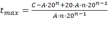
Once t max was calculated, if it exceeds 20 years (see Section 1.3.1), it was recalculated using equation (2), where the value of t was also cleared and the following expression was obtained: See (15)
Representation and analysis of the corrosion function
After determination of the corrosion function (1) or (2), in order to extract the relevant conclusions, the corrosion values C(t) were calculated for each of the values of t and a graphical representation [C(t) versus t] was also made. This allowed the visualization of the evolution and trend of the corrosion process values over time and facilitated the designer to choose the most suitable finish.
It was advisable to perform the same exercise on the same graph with different values of n, to see how it could affect its variation in the final choice, including the most demanding case, that is, when the parameter n is equal to 1 (purely linear behaviour).
Application of customer restrictions and final coating selection
From the analysis derived in the previous step and the customer requirements established in step 1, the most suitable coating was selected.
Results and discussion
The following case study was chosen to illustrate the methodology described in our work. The city of Alicante (Spain), 30 meters from the sea coast, is an area with high pollution rates, with high concentrations of sulphurs [1.55 mg·(dm-2·d-1)] and chlorides [1.66 mg·(dm-2·d-1)].
Following the proposed methodology, the subsequent steps were applied:
Customer requirements
For this case study, the following requirements were taken:
Dimensions of the prescribed tray: height 60 mm and width 200 mm
A 15-year guarantee against corrosion
Determination of atmospheric data (Location)
Geographical location of the facility: Alicante (Spain), 30 metres from the sea coast.
In the case of wetness time, it was estimated as W (equivalent to the time period in which RH> 80% and T> 0 ºC). As indicated in Table 6, for the case of Alicante, the value was W = 4300 h.
In the contamination parameters (sulphurs and chlorides, Table 6), the sulphide pollution data obtained (S) was 1.55 mg·(dm-2·d-1) and the chlorine ions (Cl-) was 1.66 mg·(dm-2·d-1).
Initial calculation of annual corrosion
It was calculated using Method 4, by applying equation (6). The following variables were determined in advance:
M: as seen above, for zinc was 0.4 (m.
t w : estimated as W (criterion RH> 80% and T> 0º C). In step (2) it was determined that the value was 4.3 thousand hours per year.
f t : was obtained from t parameter using the graph of Figure 1. Applied on the graph a t value of 4.3, it gave back a value of f t = 0.7.
f c : This value was calculated from equation (7).
The values of ( and ( were extracted from the graphs in Figures 2- figure 3, by applying the values of sulphur dioxide and chlorides’ concentrations, respectively, which were obtained at the same time from Table 6. Accordingly, these values were S = 1.55 mg·(dm-2·d-1) and Cl = 1.66 mg·(dm-2·d-1). This generated the value of ( = 1.2 and the value of ( = 4.4. Thus, f c = 1 + 1.2 + 4.4 = 6.6.
The annual corrosion was calculated with Method 4, using equation (6), where, A 4 = 0.4·4.3·0.7·6.6 = 7.95 (m.
Determination of corrosivity category
from table 9, the corrosion value calculated in the previous section (A 4 = 7.95 (m) corresponded to an ISO category of C5 (corrosivity in the range of 4.2 to 8.4 (m).
Calculation of annual corrosion (A)
Since the corrosivity category was C5, the corrosion calculated using Method 4, was accepted, i.e., A = A 4 = 7.95 (m.
Determination of the parameter n
Considering the installation in a Marine atmosphere, the parameter n was set to n = 0.90 (see section 1.3.3; Tables 3-5).
Estimation of maximum coating life
The maximum duration of the coating was calculated, as expressed in the previous section, through equation (14), where A = 7.95 (m, n = 0.9 and C is the nominal thickness of the zinc layer, which was obtained from the values in Table 11:
C ez =8 (m (electroplated)
C pg =15 (m (sheet or band pre-galvanized or continuously galvanized)
C hdg =60 (m (sheet or band hot dip galvanized)
C hdgw =100 (m (hot dip galvanized wire)
Consequently, by applying (14), the following results were obtained:
tmax (ez) =1.007 years
tmax (pg) =2.025 years
tmax (hdg) =9.447 years
tmax (hdgw) =16.665 years
Since the values for the duration of corrosion were ostensibly inferior to 20 years, the application of equation (15) was not be required.
Representation and analysis of the corrosion function
The corrosion function that followed the present case study was:
C = 7.95·t 0.9
In Table 12, the corrosion function was developed in two ways, in order to show how n-parameter can affect the final calculation:
When n = 0.9 (Corrosion C)
When n = 1 (Linear corrosion), eliminating the logarithmic component
Table 12: Annual corrosion values for logarithmic and linear functions (Alicante, Spain).
| Year | Corrosion C (µm) | t max | Linear corrosion (µm) |
| 1 | 7.95 | t max(ez) (8 µm) | 7.95 |
| 2 | 14.84 | t max (hdg) (15 µm) | 15.90 |
| 3 | 21.37 | - | 23.85 |
| 4 | 27.68 | - | 31.80 |
| 5 | 33.84 | - | 39.75 |
| 6 | 39.88 | - | 47.70 |
| 7 | 45.81 | - | 55.65 |
| 8 | 51.66 | - | 63.60 |
| 9 | 57.44 | t max (hdg) (60 µm) | 71.55 |
| 10 | 63.15 | - | 79.50 |
| 11 | 68.81 | - | 87.45 |
| 12 | 74.41 | - | 95.40 |
| 13 | 79.97 | - | 103.35 |
| 14 | 85.48 | - | 111.30 |
| 15 | 90.96 | - | 119.25 |
| 16 | 96.40 | t max (hdgw) (100 µm) | 127.20 |
| 17 | 101.81 | - | 135.15 |
| 18 | 107.18 | - | 143.10 |
Applications of customer restrictions and final coating selection
For example, the price of a mesh cable tray (made in wires), considered within the dimensions required in the project requirements (60 x 200 mm), resulted in 31 € ∙ 𝑚 −1 (Schneider Electric, 2015). If this price was divided between its average thickness (100 μm), the cost per μm was of 0.31 € ∙ (𝜇𝑚∙𝑚) −1 .
If the parameter n was not taken into account and the corrosion was understood as linear, for a 15-year guarantee on corrosion, the cost per meter of the tray was 119.25 μm·0.31 €/(μm·m)-1. i.e., 36.96 €·m-1. On the contrary, if the logarithmic factor was taken into account, the cost was 90.96 μm·0.31 €·m-1. i.e. 28.19 €·m-1.
In total, there was a difference of 8.76 €·m-1 savings, which implied a really important and positive economic impact.
Figure 5, shows the annual evolution of corrosion, with and without logarithmic function.
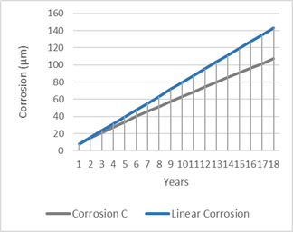
Figure 5: Comparison of annual evolution of corrosion with a linear behaviour (Alicante, 30 metres from the sea coast).
Table 12 as well as figure 5, can be very useful for the engineering and design functions since they allow to see in an analytical and visual way, the evolution of the corrosion and consequently, make it possible to optimize the type of coating and its cost.
Since the requirement was to guarantee the installation against corrosion for a minimum period of 15 years, from table 12, it can be seen that such requirement could only be met by a cable tray with a minimum coating of 90.96 μm which, going to standard thicknesses values, corresponded to a 100 μm tray, i.e. a tray made of wires, also known as a mesh cable tray, whose calculated corrosion resistance time was t max = 16.665 years. Moreover, the nominal thickness of the same tray, could be reduced to 90.96 μm, or in other words, a reduction in costs of approximately 10%. Also, the resulting environmental impact on the coating process must be mentioned, since: (1) there is less material and energy consumption (reduced thickness) and (2) lower CO2 emissions into the atmosphere.
From the results of the previous section, the optimum selection for the atmospheric conditions corresponded to a mesh cable tray with a minimum thickness of 91 μm or another type of tray with the same prescribed dimensions that would allow an equivalent finish and thickness, which in turn can comply with the economic constraints of the industrial project.
Conclusions and further research
A concise review was presented for the calculation methods for short, medium and long-term zinc atmospheric corrosion predictions. The results obtained, as well as the analysis of the study, showed that:
The calculation for medium and long-term corrosion accepted by most researchers today, followed the model established in the equation: C (t)= A·t n (1)
For the calculation of the annual corrosion, A, the methods analysed that best fitted the actual corrosion values were Method 1 (Process 3) for rural atmospheres and Method 4 (Process 6) for contaminated atmospheres
Selection of parameter n was key in the calculations and it was highly dependent on the environmental conditions of the location.
Type values and general recommendations are given for the determination of n, based in the specialized literature and research studies.
The corrosion function, especially in the first 10 years of exposure, showed a logarithmic and non-linear behaviour
A selection methodology flowchart (Figure 4), supported by a case study has been provided, based on the mathematical algorithms analysed for the calculation of A and the determination of n-parameter. This methodology involved calculating the estimated lifetime for certain atmospheric conditions and considered the different standard zinc-coated cable thicknesses currently marketed.
The fact that the evolution of the corrosion obeys exponential laws, caused the cost rate of the installation, obtained by the cost per metre of tray quotient and its thickness, to also decrease exponentially as the thickness was increased. This means that, with small increments in thickness of the coating, it is possible to exponentially increase the duration of the coating.
Consequently, the duration is much greater in comparison to the extra cost to which this increase of thickness leads to. With this in mind, it can be assumed that when using conventional techniques in many cases, installations with unnecessary costs could be prescribed. This aspect is especially relevant in cases where the parameter n moves away from the unit (rural areas or pollution-free), because the behaviour of the corrosion rate is less linear in the first years of exposure. Likewise, the reduction of the thickness required for the same duration is guaranteed, minimizing environmental impacts (material and energy consumption, emissions, among others).
This research study focused on zinc, as it is the most widely used coating in the field of electrical trunking systems. The extension of this optimisation methodology to other types of coatings will be the aim for further research, based on the methodological procedure provided in this contribution.

