


 Spanish (pdf)
 Article in xml format
 Article references
 Send this article by e-mail
 Cited by SciELO
  Similars in
SciELO
Similars in
SciELO 
 Permalink
INTRODUCTION
The demand growth is a constant concern for Transmission System Operators (TSO). To address this situation, TSOs require expansion plans to establish measures to fulfill the demand projections while maintaining power quality parameters. In these future network requirements, besides planning the renewal or the addition of power plants, it is also mandatory to consider the grid’s reinforcement to make sure that the network can transfer this new generation without compromising the power system stability [1], [2],[3].
Another concern for the operator is the system’s operation after a contingency. In the case of a fault on High Voltage (HV) networks with radial topology, the system’s voltage stability is affected due to the lack of paths to transfer the generated power. The construction of parallel lines could be a solution to this problem. Besides increasing the power transfer capacity of the network, it could also improve reliability in post-fault scenarios, preventing the disconnection of power plants and maintaining the reactive power reserves. However, because of the long-term investment it represents, TSOs look for more economical alternatives. For example, countries such as Chile [4] and South Korea [5] have reported avoiding that kind of investment by installing significant amounts of reactive power compensation in the most vulnerable zones of the circuit to a voltage collapse. It is a more reasonable solution since it is cheaper and provides more stability and transfer capacity in the power system.
Different methods are proposed in the literature to assess the voltage stability in power systems. For example, four widely used methods are the QV Modal Analysis, QV Sensitivity Analysis, and the PV and QV curves. The reason behind the use of these methods is that they require static power flows to develop the analysis. However, each method has different purposes and distinct application advantages as well as disadvantages.
The QV Modal and the QV Sensitivity Analysis are similar methods. Both of them require as input the inverse matrix of the resulting Jacobian from the power flow. The difference between these methods is that the QV Modal Analysis calculates the matrix eigenvalues to determine whether a specific bus is stable [6]. Instead, the Sensitivity Analysis determines the stability of a bus by looking at the bus’ respective value on the diagonal components of the matrix. This value corresponds to the sensitivity of the voltage in the bus with respect to the change in the reactive power [7]. Both methods check for the sign of the observed value; if it is positive, then the bus should not have voltage instability problems.
On the other hand, PV and QV curves are graphical methods based on the results obtained by a sequence of power flows in which the voltage levels are continuously tracked. The PV curves determine the power transfer limit between generation and load zones by incrementing the generated power in each simulation until unstable operating points appear [8]. Alternately, QV curves are in function of the increment of the reactive power injection/consumption in a single bus until reaching voltage levels that are not within an acceptable range. This characteristic helps to determine the reactive power requirement of some specific buses in the circuit and how would the voltage level change according to the reactive compensation [9].
Among the exposed methods, QV curves, QV Modal, or QV Sensitivity analyses are more suitable for identifying and localizing vulnerable zones to voltage instabilities. Even though the last two methods are considered to be more straightforward since the results are obtained directly from the matrix and not from a number of power flows, these methods have the disadvantage that they are not available in all the simulation software, or at least in some cases, it is required an external program, for example, Matlab, to extract the information to develop the analysis. Another problem that these two methods have is that depending on the size of the network, the computational effort to invert the Jacobian matrix is a topic of concern [10].
QV curves have many application advantages over the other methods. It is a fast method compared to dynamic studies, and unlike PV curves, it has fewer problems when it comes to convergence [11]. Also, it is a widely used tool: Recent studies have reported using simulation software such as PSSE [12], DigSilent [13], PowerWorld [14], NEPLAN [15], Matlab [16], and Python [17] to develop QV curves in real and test circuits. The analysis of these curves, and if possible, complemented with other voltage stability criteria such as modal or sensitivity analysis, helps to study the reactive power margins, determine the most suitable areas to install reactive compensation, and make planning decisions in the long and medium term.
Authors in [11] suggest that the results obtained from the QV curves in post-fault scenarios must be complemented with dynamic simulations. The traditional way to obtain the QV curves does not contemplate the evolutionary behavior of On Load Tap Changers (OLTC), Overexciting Limiters (OEL), Governors, and Automatic Voltage Regulators (AVR) during a fault and their effect on the system, which can guide misleading conclusions. Hence it opens the door to inaccurate reactive power compensation sizing and locating. Since then, no further research has been related to a proposal that improves the reliability of the results of the QV curves in the post-fault state.
This paper addresses a different way to obtain the QV curves in a post-fault state by assessing the operating points resulting from dynamic simulations instead of the contingency power flow using a model of a real large-scale circuit. This methodology evades the disadvantages of QV curves exposed by [11]. Moreover, by taking the stabilized operation points after dynamic simulations to create the QV curves, it complies with the premise exposed in [8] by characterizing the steady-state operation of the system. The main contributions of this paper are:
Providing a reliable methodology to obtain QV curves for post-fault scenarios to be applied on a real large-scale network model, contemplating the effect of dynamic elements such as the different OELs and OLTCs.
Determining zones prone to voltage instability due to the presence of faults. So that these are later reinforced through the amount of reactive compensation specified on the QV curve and help mitigate voltage instability problems.
The remainder of the paper is organized as follows: Section 2 presents the classic formulation of the QV curves, and Section 4 describes the proposed methodology in this study. Section 4 shows the planned expansion in Argentina for 2024 and the need for voltage stability studies. The QV analysis for the Patagonian HV network is presented in Section 5. Finally, the Conclusions and Future Work are presented in Sections 6 and 7, respectively.
QV CURVES
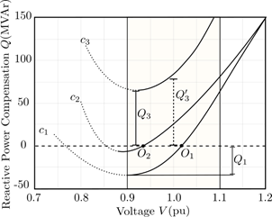
QV curves depict the reactive power, consumed or injected, needed to obtain a specific voltage level in a bus. When plotted, the x-axis corresponds to the voltage level, and the y-axis to the reactive power compensation. The positive sign in the y-axis is associated with reactive power injection and the negative sign with consumption. Fig. 1 shows an example of three different QV curves c 1 , 𝒄 𝟐 and 𝒄 𝟑 in the voltage range of 0.7 pu to 1.2 pu.
The curve divides into two operating zones according to the slope of the curve: stable (positive slope, the solid line in Fig.1) and unstable (negative slope, dotted line). The unstable part of the QV curve corresponds to deficient voltage levels, which are undesirable operating points. Instead, the stable side corresponds to voltage levels comprehending a range of acceptable values.
Each curve’s knee point reveals the correspondent bus’s reactive power margin. This point also informs from what value of reactive power the operation is in the stable zone of the curve. If the margin is negative, there exists at least an operation point on the stable zone of the curve. On the contrary, if the margin is positive, there is no operation point without the injection of reactive power (installation of capacitive compensation).
Fig. 1 depicts the margins for curves 𝒄 𝟏 and 𝒄 𝟑 through the values 𝑸 𝟏 and 𝑸 𝟑 , respectively. In the case of 𝒄 𝟏 , it shows that the curve has a range of 𝑸 𝟏 MVAr, where an operating point in the stable zone is ensured until reaching the point 𝑶 𝟏 . On the other hand, 𝒄 𝟑 corresponds to a curve with a positive margin, a typical curve of very loaded scenarios. To guarantee an operating point on the stable side of the curve, the bus needs the injection of at least 𝑸 𝟑 MVAr. However, the knee point of the curve is not always associated with a voltage value in an acceptable range, so a higher compensation is required. Thus, to ensure a 1.00 pu voltage operation at the bus, 𝑸 𝟑 ′ MVAr should be installed, a value greater than 𝑸 𝟑 .
The methodology to get the curve consists of installing a fictitious generator with no active power generation and without reactive power limit in the bus of interest and then running a series of power flow simulations. The bus changes from PQ to PV type, setting the voltage value in a specific range through the power flow series to obtain the reactive power injection/consumption to hold the voltage level at the specified value.
Different ways exist to execute the power flow series for obtaining the QV curves. One method starts with identifying the base voltage value from the original power flow. Then, the simulations could be performed in two sequential stages: ascending, beginning from the base voltage and increasing it in small steps until reaching the established upper limit, then descending from the base voltage to the lower limit.
In post-fault scenarios, to contemplate the operation of an isolated area by a three-phase fault, the bus with the highest rated capacity in the islanded system is selected as a slack bus, allowing the power flow to reveal the voltage level status of these zones.
There are some considerations regarding the voltage range of the curves. When evaluating high or low voltage values, there exists the risk that the power flow does not converge. Researchers in [18] used the PSSE software to perform a QV analysis using the non-divergent power flow option, which ensures obtaining values that, despite not being convergent, avoid unrealistic results by stopping the simulation before getting very high mismatches. On the other hand, in [1] and [19], they avoid the convergence problem using the Continuation Power Flow method. The most conservative way to deal with this problem is taking the recommendation from [9], which suggests that the most relevant voltage range is between 0.9 pu and 1.1 pu. Although when evaluating only in this range of values, the complete behavior of the curve is not shown, it may be enough to detect voltage instabilities.
PROPOSED METHODOLOGY
The classical way to develop QV curves for post-fault scenarios is through contingency power flows. These simulations are based on a static power flow (i.e., Full Newton Raphson) in an N-k status network. As stated previously, this procedure does not contemplate the action of control mechanisms which could be essential for supporting voltage stability when a contingency appears. This simplification could lead to inaccurate conclusions, labeling, for example, voltage conditions in a bus as unstable when dynamic simulations show that they are indeed stable, as shown in [11].
A reasonable alternative for tackling this problem is taking the operating points after a dynamic simulation as a base to develop the curves. With an adequate base of dynamic models, these kinds of simulations give accurate information about the post-fault state, including the effect of the automatisms that the classic power flow cannot provide.
Using the resulting operating points from dynamic simulations means taking a snapshot of the network condition seconds after the fault is simulated. Ideally, the time between the fault and the snapshot has to be long enough so that the oscillating effect does not influence the operating points. After that, the same sequence explained in Section II to obtain the QV curve is followed for the list of buses under study.
In the series of power flows required to obtain the curves, all the setpoints obtained from the dynamic simulation are also considered: This includes the generators’ active power delivered, reactive power delivered or consumed, and voltage setpoints fixed at the resulting value. It also comprehends the transformers’ new tap positions, switched shunts’ statuses, and the load consumption according to the resulting voltage level (ZIP model).
Since the study focuses on the injection or consumption of reactive power and its effect on the voltage levels and also considering that the frequency levels after the dynamic simulation should be close to nominal, the methodology assumes the simplification of fixing the frequency base value at nominal.
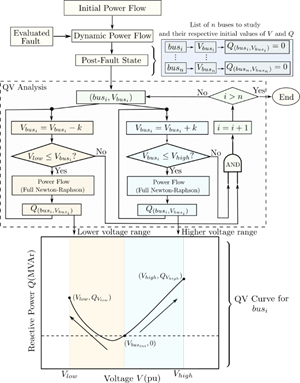
Note that the main difference between the classic method and the one proposed in this study is the choice of the initial operating points. Taking this into account, Fig.2 illustrates a diagram for the proposed methodology, where the variable 𝒌 is the size of the voltage step in the ascending and descending sequence of power flows, 𝒏 the number of buses under study, and 𝑽 𝒉𝒊𝒈𝒉 and 𝑽 𝒍𝒐𝒘 are the upper and lower voltage limits of the QV curve.
THE PATAGONIAN EXPANSION PLAN FOR 2022-2024
Due to the long extension of the country and its geography, the more abundant natural resources in Argentina vary according to latitude. In the northwest, there is more potential to exploit solar energy, whereas in the south, especially in the Patagonian region, hydro and wind power.
One of the main objectives of the expansion plan in Argentina for the medium term is to take more advantage of the resources in the Patagonian Region to supply the growing demand in the future years [20]. There are approximately 1.5 GW of wind power installed capacity, and the expansion plan sets the installation of 25 MW of wind power and 1.3 GW of hydropower capacity in two stages: 360 MW for 2024 and 950 MW for 2029.
Argentina relies on 500 kV HV networks to transport the generated power from the north and south regions to the main demand centers of the country. In the Patagonian Region’s case, a radial corridor of 1120 km goes from La Esperanza 500/220 kV substation to the Choele-Choel 500/330/132 kV substation. At that point, the network meshes for approximately 1000 km until the capital city, Buenos Aires. With the inclusion of future power plants, reinforcing the Patagonian HV radial corridor is a topic of interest for the TSO.
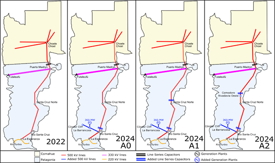
Fig. 3 depicts the 500 kV Patagonian network’s expansion plan from 2022 to 2024. By 2024, when the planned 360 MW hydropower plant in La Barrancosa station comes into operation, three reinforcement alternatives are considered: A0, A1, and A2. Alternative A0 corresponds to the original plan for 2024, which in comparison with 2022, it includes a line series capacitor after Río Santa Cruz 500/132 kV substation. Alternatives A1 and A2 are based on A0: A1 incorporates a line series capacitor right after the Santa Cruz Norte 500/132 kV substation. On the other hand, A2 contemplates the partition of the HV line connecting the Santa Cruz Norte and Puerto Madryn substations to create the Comodoro Rivadavia Oeste substation. There a line series capacitor is installed.
According to [20], the reason behind the installation of line series capacitors is to increase the power transfer in the corridor since it has saturation problems. These devices also can improve the reactive power support to maintain the voltage levels in an acceptable range. Nevertheless, when faults occur, the capacitors are bypassed [9], causing the system to run out of the reactive compensation they provide in a critical situation, aggravating the general stability of the system.
Due to the radial topology of the Patagonian system, faults on the 500 kV network could imply severe consequences for the system’s voltage stability. Single-phase faults with successful reclosing can cause back-swing problems. In addition to violating the security operation criteria for an adequate voltage level, it could generate the disconnection of loads or even cause the grid to operate in weak operating conditions. On the other hand, three-phase faults can cause the islanding of some portions of the system and the loss of availability of reactive power sources to maintain voltage levels. However, for this kind of fault, there are resources such as the automatic disconnection of generators through System Protection Schemes (SPS) to balance the demand and the generation in an N-1 system condition. Another possible consequence, depending on where the fault occurs, is that the power flow intended to be transported by the 500 kV network diverts to the adjacent 132 kV network through the Santa Cruz Norte substation, overloading the lower-voltage network and aggravating the voltage problems in the area.
CASE STUDY
System description
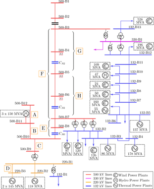
Fig. 4 shows a single-line diagram of the Patagonian HV network scheduled for 2024, including the elements of the three reinforcement alternatives and the adjacent 132 kV part connected to the 500 kV Network between Puerto Madryn (500-B3) and Santa Cruz Norte (500-B7) substations. Due to the voltage impact that the 132 kV network may suffer as a consequence of a fault, it is necessary to consider it to get a better perspective of the stability of the whole network.
Post-fault Scenarios
The letters from A to G in Fig.4 denote the eight fault locations to be considered. Each letter is associated with the line to fault. It must be noted that locations G and H are exclusive for alternative A2 since substation Comodoro Rivadavia Oeste (500-B5) splits the 500 kV line from Puerto Madryn (500-B3) to Santa Cruz Norte (500-B3). Consequently, location F is only considered by alternatives A0 and A1. The other fault locations are part of all three alternatives.
Only three-phase and single-phase faults with successful reclosing are studied regarding the types of faults to be simulated. Three-phase faults are considered in all of the described locations in Fig.4, while single-phase faults are considered only for locations F, G, and H due to the effect of this type of fault on the main 500 kV corridor (500-B3 to 500-B7) could be detrimental.
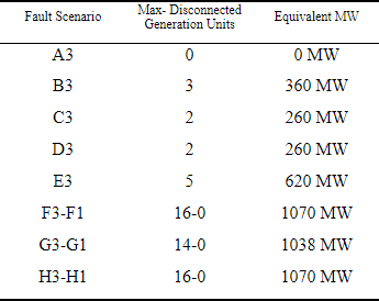
When evaluating three-phase faults, the automatic disconnection of generation units is considered. Table 1 shows the maximum number of disconnected generators and the corresponding total amount in MW for each fault location and type of fault (3 for three-phase and 1 for single-phase faults). In the case of single-phase faults, the disconnection of generating units is not considered.
Besides contemplating different fault locations and the automatic disconnection of generation units, the post-fault scenarios consider four distinct generation cases that depend on the power delivered by the principal power plants in the area: La Barrancosa (500-B11) and Río Turbio (220-B3). These are:
0G: All generators are turned off (P = 0 MW).
0G-RT: Generators of 500-B11 are off, but those of 220-B3 are delivering power at 50% of their nominal capacity (P = 140 MW)
3G: All generators of 500-B11 are at 95% of their nominal capacity, and those of 220-B3 are off (P = 342 MW).
3G-RT: Generators of 500-B11 and the ones of 220-B3 are at 95% and 50% of their respective nominal capacity (P = 482 MW).
Previous considerations for the QV curves
The dynamic simulations and the QV curves were made using PSS/E software version 33.5 and the Python programming language.
The initial operation points to use in QV curves were obtained from the result of dynamic simulations. The dynamic models used are the homologated ones from the network under study. These simulations considered a time window of 900 s (15 minutes) after the simulated fault. At the end of the simulation, if the operating points are in a steady-state condition, then this point is taken to develop the QV curves of the corresponding case.
The ZIP model considered the load model for the dynamic simulations and the QV curves, where the current and impedance constant proportion for the active power part was 80% and 20%, respectively. Instead, the reactive power part was 50% - 50%.
The QV curve slope and the base voltage value when the reactive power is 0 determine if a bus tends to have voltage problems. If the bus voltage value in the post-fault cases ranges from 0.95 pu to 1.05 pu for buses in the 500 kV network or from 0.93 to 1.07 for the 132 kV network, the bus does not tend to have voltage problems. Otherwise, the bus requires reactive power compensation to improve the voltage conditions. On the other hand, the QV curve slope determines the increment ratio of reactive power injection with respect to voltage. If this ratio is high, it could be a problem since high compensation sizing would be required to achieve small changes in the voltage level, which depending on the compensation device, is not always physically possible.
Results
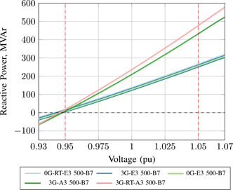
Figs. 5, 6, and 7 show the QV curves for the alternatives A0, A1, and A2, respectively, exposing only the buses in different generation and fault location scenarios whose voltage is lower than 0.95 pu for 500 kV buses or 0.93 for 132 kV buses when the reactive power consumed/injected is 0. Neither of the analyzed cases presented a base voltage above 1.05 pu.
For the case of the curves shown for alternative A0, voltage problems occur in bus 500-B7 for two specific fault locations: A3 and E3. The base voltages of all the scenarios are slightly lower than 0.95 pu, meaning that they require low reactive compensation. However, the slope of the curve reveals that faults in location A are more problematic than faults in location E, requiring more reactive compensation than the other case to maintain the same voltage level.
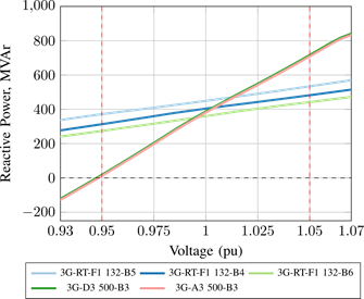
In the curves shown for alternative A1, bus 500-B3 presents voltage problems in the 3G generation scenario for three-phase faults in A and D, similar to those in scenario A0. Nevertheless, the attention is on the single-phase fault with successful reclosing at location F in the higher generation scenario (3G-RT). The 132-kV buses 132-B4, 132-B5, and 132-B6 show a different problem: they have a low slope but require more reactive power (from 200 to 600 MVAr) to have an operating point between an acceptable voltage range.
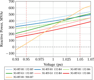
In alternative A2, the same group of 132 kV buses reported similar voltage problems when evaluating the 3G-RT scenario for single-phase faults with successful reclosing in locations H and G. When the fault is assessed on location H, the required compensation ranges from 270 to 550 MVAr. In contrast, location G varies from 145 to almost 500 MVAr. Also, bus 500-B7 presented voltage problems similar to the ones reported in A0: base voltage close to 0.95 and high slope.
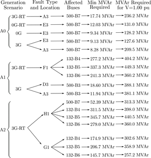
Fig. 8 shows a results diagram detailing each case with voltage problems in the three alternatives according to the generation scenario, fault type, and location. It also includes the minimum reactive power compensation required to have a voltage value between acceptable ranges depending on whether the bus is on the 500 kV or 132 kV network and the required compensation to reach a 1.00 pu voltage.
The results show that each alternative has localized and common areas where voltage problems occur in different fault and generation scenarios. In the case of alternative A0, the issues are in bus 500-B7. While in alternatives A1 and A2, the problems mainly occur in the 132 kV buses: 132-B4, 132-B5, and 132-B6.
Also, in terms of the need for reactive power compensation, the post-fault scenarios with the highest generation after a single-phase fault with successful reclosing in the 500-B3 to 500-B7 corridor are more problematic than three-phase fault scenarios. For each of the reported 132 kV buses with voltage problems for these cases, the base voltage values are lower than 0.93 pu and require almost 150 MVAr to 345 MVAr of compensation to have acceptable voltage levels. It is worth noting that in both planning alternatives, bus 132-B5 requires more compensation than the other 132 kV buses.
CONCLUSION
This paper assessed the QV curves using the post-fault network operation points obtained from dynamic simulations under different generation and fault scenarios. The results identified zones prone to voltage instability and the approximate amount of reactive compensation necessary to solve the problem in the Patagonian HV network under different planning alternatives.
Three planning alternatives for the year 2024 were evaluated. The QV curves of each of these alternatives showed a certain similarity, identifying the 500 kV area of Santa Cruz Norte (500-B7) and part of its extension at 132 kV (buses 132-B4, 132-B5, and 132 -B6) as areas prone to voltage instability.
In the cases studied, a pattern was noted for the two types of faults analyzed. The QV curves for scenarios where three-phase faults were evaluated generally showed base voltage values close to the lower allowable limit with a high slope. On the contrary, single-phase faults with successful reclosing for alternatives A1 and A2 showed the need for more significant reactive compensation than three-phase fault scenarios to achieve an operating point in an acceptable range.
It is not possible to define a specific amount of reactive compensation that works for all the post-fault scenarios evaluated in the three planning alternatives. However, it was demonstrated that QV curves could give an insight into a range of possible values, which would depend on the evaluated case.
FUTURE WORK AND RECOMMENDATIONS
The proposed methodology can be extended to analyze other transmission systems. Nevertheless, it is important to remember that each network has its own characteristics, and the results obtained in this study cannot be extrapolated to other similar networks.
By identifying the location of the most vulnerable areas to voltage instability and the approximate necessary size of the reactive compensation needed, it is now possible to assess the type of element that will have such work.
Flexible Alternating Current Transmission Systems (FACTS), specifically the Static Synchronous Compensator (STATCOM), are gaining a good reputation worldwide for solving voltage instability problems. STATCOM devices can improve the power transfer, support the network under critical conditions better than shunt capacitors, and do not depend on the voltage level of the point of connection to inject/consume reactive power with a fast response. With the employment of this kind of element, the effects of faults on the voltage levels can be mitigated, ensuring better reliability.
Future research aims to evaluate the use of STATCOM on the Patagonian Network through dynamic simulations. The WECC-validated generic model SVSMO3 and the simplified CSTCNT models can be employed for such labor in PSS/E.

