


 Inglés (pdf)
 Articulo en XML
 Referencias del artículo
 Enviar articulo por email
 Citado por SciELO
  Similares en
SciELO
Similares en
SciELO 
 Permalink
1. Introduction
Several studies have been conducted in order to describe potential factors that might explain the behavior of the wages in an economy. Mainly, the Mincer earnings function1, Jacob Mincer (1974), has been applied to different samples, even to various countries and industries. Moreover, in the sports industry it would be interesting to develop a model that enable us to describe how experience interacts with wages of sportsmen, specifically, the NBA players’ wages.
However, frequently the models used to investigate this equation stand on many assumptions, in some cases really strong (e.g. exogeneity, homoscedasticity, etc.) and violations to these assumptions can affect, to some extent, the conclusions derived from these models. Nonetheless, it is important to mention that there is plenty of bibliography related to techniques that allow researchers to overcome many estimations problems that might arise from the violation of these assumptions2.
The main reasons why a model estimated using a technique of estimation that relies on assumptions can lead to wrong conclusions (due to not fulfillment of these) can be: a) heteroscedasticity, which underestimates the variance of the coefficients; b) not normal distribution of the error terms, which also affects the variances of the estimates; c) autocorrelation; d) endogeneity; among others. Thus, statistical inference will present skewness. Specifically, the confidence intervals of the fitted values of the dependent variable won’t be precise.
Fixing the specification issues that an OLS estimation might present can be burdensome, therefore, as an alternative, a nonparametric estimation, e.g. using a k nearest weighted neighbor, is proposed to get more reliable confidence intervals without the need for further corrections to the original estimation method.
In particular, in the present work we are interested in showing how a nonparametric estimation represents appropriately the shape of the relation of the logarithm of the wages of a sample of players of the NBA and their years of experience. Furthermore, a confidence interval is estimated from the nonparametric estimation in order to pursue reliable statistical inference. Additionally, the obtained results are compared to the classical OLS estimation, in which we also included the years of experience squared in order to have no constant relation in the model. As a result, it can be seen that all assumptions of the OLS estimation are violated, so that the confidence interval presents problems.
2. Data and descriptive statistics.
The econometric modelling of wages is usually based on the assumption that a person’s pay is correlated to their personal skill. Nevertheless, since direct measures of the level of skill are hard to find, most models tend to approximate it by the level of education, IQ or (like in the present paper) the level of work experience. Sports are a field of study that allow for specific measures of work performance and empirical studies lead to the result that better performing athletes tend to earn more money (Rose, S., Sanderson, A., 2000). Taking into consideration these reasons, we decided to perform the model comparison for a dataset that contains 267 observations3 of the NBA professional players. Specifically, it has information of annual salary and years of experience at the time that the information was gathered. It is important to note that in this particular dataset the years of experience are measured as a discrete variable. Table 1 summarizes the principal statistics of the sample.
Table 1 Descriptive statistics of data.
| min. Value | max. Value | mean | median | mode | standard Deviation | |
| Salary | 1.500.000 | 57.400.000 | 14.189.000 | 11.860.000 | 1.500.000 | 9.879.219 |
| Experience | 1 | 13 | 5,0262 | 4 | 2 | 3 |
Source: The Authors.
The range of the data is really large, for salaries is 55900000 and for years of experience is 12. Furthermore, based on the variance coefficient, the annual salary has a variation with respect to the mean of 69,63% and the wages have a dispersion of 64,42%.
Additionally, from table 2 we could affirm that, since there not many observations of the players with 12 and 13 years of experience, the estimates for this part of the dataset might have a large variance. Moreover, the low number of observations for higher level of experience suggests that the extreme fitted values may be underestimated with the nonparametric algorithm.
Readers might feel that the data is not ideal, however, it is important to remark that the purpose of this work is to compare efficiency of estimates rather than finding specific economical results.
3. Methodology.
3.1. OLS estimation.
The first model that is studied is a simplification of the Mincer function:
 (1)
(1)
Where  represents the logarithm of the wage of player i and
  the years of experience and
  represents the error term of observation i. The model is estimated with classical OLS.
The reason why we reduced the original equation is because we preferred to keep this work more parsimonious to facilitate the analysis and comprehension of the estimation method. Nevertheless, upcoming studies will have deeper analysis in which other variables (like years of schooling) are included to the equation in order to test the robustness of the results.
About the model, it has been broadly discussed whether the Mincer function is too simplistic. Even though the quadratic variable enables the model to have a variation that depends on the magnitude of the independent variable, for example, Lemieux (2003), shows that higher order polynomials enhance the capacity of prediction of the model.
Several tests are also applied in order to prove whether the estimated equation fulfill the assumptions on the classical OLS estimation. Specifically, we test the normality of the residuals with the Jarque-Bera test, the autocorrelation of the residuals using a Durbin-Watson test, and we use the White test to analyze heteroscedasticity in the model.
Finally, an asymptotic confidence interval is computed. The aim of this, is to compare this interval to the resultant from the nonparametric regression. A MonteCarlo simulation was undertaken for this purpose4.
The simulation consists on repeating the estimation process thousands of replications. For each iteration, a new dataset is generated from the original sample, so that the characteristics of the original data are kept. Afterwards, in each replication the fitted dependent variable is computed. Finally, the 0,025 sorted fitted value is taken as the asymptotic lower limit interval and the 0,975 is considered the upper limit interval. These values are considered due to a significance level of 5%.
3.2. Nonparametric estimation.
In the second part of this work we present an estimation of  using a nonparametric regression model:
 (2)
(2)
We apply the k-nearest neighbors regression technique, which takes averages in neighborhoods  of a point x. We selected this technique because, even though it is easy to implement, it exhibits remarkable flexibility while modeling low dimensional data (Altman, N. S., 1992). The neighbors are defined in such a way as to contain a fixed number k of observations (which means that we are not necessarily using the same bandwidth for each of the bins).
We find the k observations with  values closest to
  , and average their outcomes. Basically, the idea is that if
  is relatively smooth, it does not change too much as x varies in a small neighborhood. Afterwards, taking an average over values close to x,
  should give an accurate approximation.
 (3)
(3)
Where the are the realization of the k observations in which is smaller. In the case in which there are several with the same  and adding those to the previously selected observations would lead to a number higher than k we apply the following algorithm:
Divide the observations that satisfy the conditions mentioned above in two vectors, based on the sign of
 .
.Randomize the order of the elements of each of the vectors, to avoid following a pattern that might generate additional BIAS in the estimations.
Combine those two vectors into a new one, created by intercalating the first element from each vector as long as it is possible, and then the remaining elements of the vector with the higher number of observations (if necessary).
Select the remaining number of observations for
 from the first set of elements of this vector.
This algorithm guarantees that we are not over-representing players with more (or less) experience than the bin value of x, unless it is strictly necessary due to the data set used. It is necessary to implement it because of the discrete nature of the variable x, that implies that (in case we do not have a clear aleatory criterion for data selecting in certain situations) we might be systematically selecting more players with more (or less) years of experience than the estimation point, leading to BIAS that could have been avoided.
It is important to notice that the selection of k can dramatically change the outcome of the model in different ways. For example, if k = n, we are using all the observations, and just becomes the sample average of . Graphically, we will have a perfectly flat estimated function. Furthermore, a large k leads to a relatively low variance, nonetheless, the estimated is biased for many values of x, thus, the estimation is inconsistent. Whereas when k = 1 we are using one observation to estimate the value of each bin. This dramatically reduces the bias but, as we are using few observations, the variance is high.
The literature formally does not stablish a way to select an optimal value of k, however, one possible appropriate way would be by trying different values of k and picking the one that minimizes the Cross Validation estimate of the MSE (Henderson, D., Parmeter, C., 2015).
In our case we choose k using as a reference the choice presented in the section 9.4.2 of Cameron, A. C., & Trivedi, P. K. (2005) which is a value such that:  .
.
Since the intuition behind the k nearest neighbor methodology is that objects close in distance are potentially similar, we decided to apply the distance weighting refinement. We choose the Euclidian distance metric defined as:
 (4)
(4)
In order to use this distance as weight for each of the  , we decided to use the exponential weighting defined as:
 (5)
(5)
After applying the distance weighting refinement, the estimate for  is replaced for the following equation:
 (6)
(6)
Additionally, it is important to note that, since the x (years of experience of the player) are discrete variables, it is essential to take this into consideration while choosing the number and location of each bin in order to avoid creating skewed neighborhoods.
4. Results and Discussion.
First, model (1) was estimated with OLS. The result of this estimation is presented in table 3.
We can see that all the coefficients are significant. Furthermore, the signs of the estimates for years of experience and for squared years of experience are as expected, given that the curve of this equation is concave.
However, this model presents: not normal residuals, positive residual autocorrelation and heteroscedasticity, as the tests shows. Consequently, based on classic econometric theory, we can affirm that the variance of the estimates won’t be efficient. Therefore, statistical inference, and more precisely, the confidence interval is not reliable.
Indeed, from figure 1, it is easy to realize that at the extreme, the intervals start to explode away from the fitted values.
Secondly, we estimated the k nearest neighbor regression, using distance weighting. As this model is sensitive to the value of k, we ran it for different values of this parameter in order to graphically asses the tradeoff between BIAS and variance that was describe in the methodology section. The comparison of these results can be seen in section 7.1. The k nearest neighbor regression for different values of k. After applying this procedure we selected k = 65. It is important to remark that the ratio of the selected is between the ratios of the ks recommended by Cameron and Trivedi (0.05 and 0.25).
As it was mentioned in the Methodology section, before estimating the model, it is necessary to take into consideration that the variable “Years of experience” follows a discrete distribution. A discrete distribution of x implies that an arbitrary placement of the bins will lead to additional problems in the model outcome. This is due to the fact that (since many of the observations consist in the same value of x) a bin placed in a certain position (e.g. ) will have the same k nearest neighbors as a bin placed relatively far away (in this example the furthest bin with the same neighborhood will be close to ). This is one of the reasons why we decided to use the distance weighting5 refinement that partially solves the problems that may arise from this situation. The problems are mitigated because, in spite of the fact that both bins have the exact same k nearest neighbors, the weights for each observation will vary based on the value of and therefore will change as well. Nevertheless, we decided to place the bins either for or 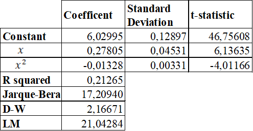 where a is an integer, in order to guarantee that each bin is associated to a different neighborhood.
Now we present the results from the k-neighbor regression for k = 65 with the corresponding confidence intervals computed through bootstrapping:
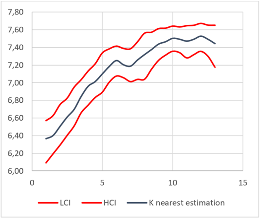
As it can be seen in figure as the relationship captured by the non-parametric technique applied leads a result that resembles a logarithmic relationship between the variables considered. It resembles the logarithmic function in the sense that it grows at a higher rate in the first years of experience and after some years it starts to grow at a decreasing rate. Nevertheless, there are two main differences when we compare it to a logarithmic function.
The first one is that at the beginning of the function the growth rate is relatively small. This is one of the characteristics of the k nearest neighbors algorithm because (since a lot of the nearest neighbors for 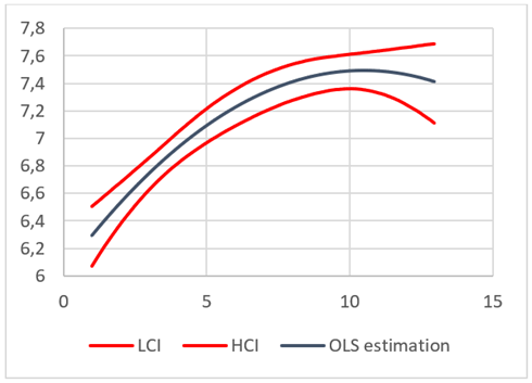 are related to
  and non are related to
  ) the first bin usually leads to overestimation of
  .
.
The second difference is found for  , that yields an estimate
  that is smaller than it should be for a logarithmic function. After analyzing the data set, we realized that there are not many observations for x = 7, which might lead to a significant difference between the sample distribution and the population distribution of the variable. Additionally, as it can be seen in the confidence intervals for x = 7, the lack of observations in this point also increases the amplitude of the interval.
The first difference is inevitable and inherent to the estimation technique used, but the second one could be solved by utilizing a bigger data-set. Additionally, it is important to note that (similarly to the case of the first bin) the last bin tends to be underestimated since it is a function of observations associated to lower levels of experience.
4.1. Comparison between the models
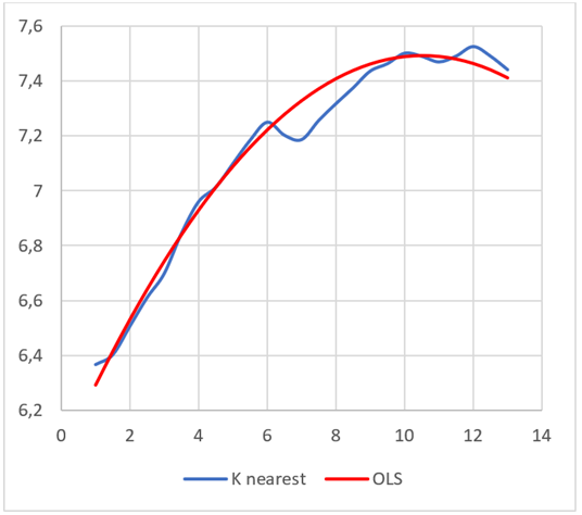
Both the estimates that comes from the OLS and the K nearest neighbors are remarkably similar. We detect three main differences:
The K nearest estimation is higher in the first bins. This is probably due to the fact that this algorithm tends to overestimate the first bins.
Close to x = 7 we see that the K nearest estimation suddenly lowers its value but later it returns to values similar to those of the OLS. As it was stated in the previous section, this is probably a feature of the data that could be solved if the data set could be expanded. There is no theoretical reason for this and since both functions behave similarly for the following values of x, this is probably just an issue with the dataset.
For the last bins, the OLS estimation is lower than the K nearest one. Since the K nearest neighbors algorithm tends to underestimate monotonically increasing functions in the last bins, could be an indication that the OLS is underestimating the function even more.
5. Conclusions
Both estimation techniques yield similar outcomes for the dataset analysed. Nevertheless, the lack of assumptions behind the K nearest neighbors algorithm makes it easier to implement, especially in a context in which the OLS violates several assumptions. Not addressing the assumption violation in the OLS can lead to underestimating the variance of the coefficients, rendering the model unable to perform trustworthy inference. Addressing these problems might be time intensive and troublesome. This paper exhibits the K nearest algorithm with the distance weighting refinement as an alternative, due to results presented in previous sections, that might provide fewer estimation issues and lead to similar results. Additionally, there is evidence that this model might perform better than the OLS for players with more than 11 years of experience. It would be interesting to conduct a study that could provide further evidence in this matter, especially if the dataset analysed contains players with more than 13 years of experience.


