


 Español (pdf)
 Articulo en XML
 Referencias del artículo
 Enviar articulo por email
 Citado por SciELO
  Similares en
SciELO
Similares en
SciELO 
 Permalink
Forma sugerida de citación:
Montero, S.; Bustamante, R.; Ortiz-Bernardin, A. (2018). «On the behaviour of spherical inclusions in a cylinder under tension loads». Ingenius. N.° 19, (january-june). pp. 69-78. doi: https: //doi.org/10.17163/ings.n19.2018.07.
1. Introduction
In Refs. [1–3] Rajagopal and co-workers have proposed some new types of constitutive relations, which cannot be classified as either Green or Cauchy elastic equations. If T and B are used to denote the Cauchy stress tensor and the left Cauchy Green tensor, respectively, one of such relations is f(T,B) = 0, and two special cases that can be obtained from the above implicit relation are the classical nonlinear constitutive equation for a Cauchy elastic body [4] T = g(B), and the subclass B = h(T) (see, for example, Ref. [5]).
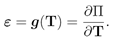
As a particular case, we assume that the gradient of the displacement field is small. From the above equation B = h(T), we obtain ε = g(T), where " is the linearized strain tensor. This last constitutive equation is very important on its own, since it could be used to model the behavior of some materials that can show a nonlinear behavior, but where the strains are small, such as rock [6, 7], concrete [8] and some metal alloys [9]. Another important use of ε = g(T) is in the fracture mechanics analysis of brittle bodies [10], where for some particular expressions for g(T), it can be proved that for a crack in a brittle body, the magnitude of the strains are limited and do not go to infinite near the tip of a crack, contrary to what happens when the classical linearized elastic theory is used (see, for example, Ref. [11]). It is very important to study the behaviour of elastic bodies considering ε = g(T) for as many different boundary value problems as possible, in order to understand the capabilities and drawbacks of these new constitutive models, and that is the main objective of the present communication.
We are interested in studying the behaviour of a hyper-elastic (Green solid) cylindrical sample that can contain 1, 2 and 5 spherical inclusions, which are located in a row in the central axis of the cylinder, and which are equally separated from each other. The inclusions are assumed to behave as nonlinear elastic solids, using the new constitutive equation ε = g(T) mentioned above. For simplicity the composite sample is modeled as an axial-symmetric body and a tension load is applied on the upper part of the cylinder. The finite element method is used to obtain results for the boundary value problem. We are particularly interested in studying the behaviour of the stresses and strains near the interface of the inclusions and the surrounding hyper-elastic body. It is assumed that the spherical inclusions are perfectly attached to the hyper-elastic matrix. The hypothesis of our work is that the new classes of constitutive equations ε = g(T) can be useful for the modelling of brittle bodies, in particular in the case we have large stresses, but where the strains must remain small. For a cylindrical sample with inclusions, such concentration of stresses appear near the interface of the matrix and the inclusion, and as it is shown in the present work, considering a particular expression for g(T), that we indeed obtain small strains for the spherical inclusions. For the modelling of such composite materials is very important to obtain results as precise as possible of the stresses near the interface, as the most common failure, which such composites show, corresponds to the debonding of the particles with the surrounding matrix.
his work is structured into the following sections. In Section 2 we present the basic equations for the models, in particular, the constitutive equations used for the spherical inclusions. In Section 3 we give details about the models to be analyzed. In Section 4, some numerical results for the different cases analyzed are presented. We end in Section 5 with some concluding remarks about the numerical results presented in this paper.
2. Basic equations
2.1. Kinematics and equation of motion
Let X denotes a point of a body B, the reference and current configurations are denoted as Br and Bt, respectively, and the position of point X in such configurations is denoted as X and x, respectively. It is assumed that there is a one-to-one mapping such that x = (X, t), where t is time. The deformation gradient F, the left and the right Cauchy-Green tensors B, C, respectively, the Green Saint-Venant strain tensor E, the displacement field u and the linearized strain tensor ε are defined as:
Respectively, where ∆ is the gradient operator with respect to the reference configuration. We assume 0 < J < ∞, where J = det F.
The equation of motion is
where ρ is the density of the body in the current configuration, T is the Cauchy stress tensor, b represents the body forces in the current configuration, ( ¨ ) is the second derivative in time, and div is the divergence operator defined in the current configuration.
In our work we consider quasi-static deformations, therefore the left side of (4) is zero. More details about the above relations can be found, for example, in Ref. [13].
2.2. Constitutive equations
We consider a body composed of two materials, a matrix which is assumed to be hyper-elastic, filled with spherical inclusions which are assumed to behave as nonlinear elastic bodies undergoing small strains. For the hyper-elastic matrix cylinder, we assume there exists a function W = W(F), called the energy function, such that (see, for example, Ref. [4])
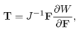
where we use the convention  In this work, we use the neo-Hookean compressible model
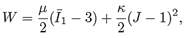
Where 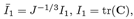 where tr is the trace of a second order tensor, and μ, κ are material constants.
For the inclusions, we assume that they are elastic bodies that develop nonlinear behavior when strains are small. As indicated in the introduction section, recently some new types of constitutive relations for elastic bodies have been proposed in the literature [1–3], one of such relations is of the form

where the Cauchy elastic body T = g(B) is a special subclass of the above relation, plus the new constitutive equation

Assuming that  then
then  (we also have E ≈ ε), and from (8) we obtain (see, for example, Refs. [14, 15])

where in general g(T) is a nonlinear function of the stress tensor. We consider a special case of (9), where we assume there exists a scalar function II = II(T) such that (see Ref. [16])
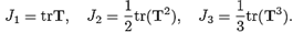
If II is assumed to be an isotropic function, we have that II (T) = II(J1, J2, J3), where Ji = 1, 2, 3 are the following set of invariants of the stress tensor
And from (10), we obtain the representation
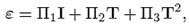
Where 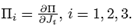
The following particular expression for II is considered:
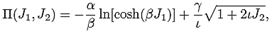
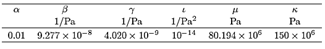
Where α, β, γ and ι are constants.
Eq. (13) has been used in Ref. [17] to study problems, where independently of the magnitude of the stresses, the strains remains small. It is necessary to point out that this form for II and the numerical values of the constant that are shown in Table 1, have not been obtained from experimental data. In Figures 1, 2 presented in Ref. [17], some plots for the behavior of a cylinder under tension are shown, where it is possible to observe that the strains remain always small independently of the magnitude of the stresses. As indicated in the introduction section, such particular expressions could be important for fracture analysis of brittle bodies. Finally, in Table 1 the numerical values of the constants used in (6) and (13) are presented.
2.3. Boundary value problems
For the hyper-elastic cylinder, the boundary value problem is the classical formulation in nonlinear elasticity, where the function χ(X) is found by solving the equilibrium equation in the reference configuration (see, for example, Ref. [4]:

Where  is the nominal stress tensor. From (5),
  and Div is the divergence operator with respect to the reference configuration. Eq. (14) must be solved using the boundary conditions

Where  is the boundary of the hyper-elastic body in the reference configuration,
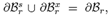
 N is the outward normal vector to the surface of the body in the reference configuration, s is the external traction (described in the reference configuration), and x is a known deformation field on some part of the surface of the hyper-elastic body.
For the inclusions we consider small strains and displacements. And following what has been presented in Refs. [16, 17], for the boundary value problem corresponds to find T and u by solving (see (3), (4) and (10))
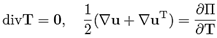
simultaneously. In the above system we have 9 equations for a fully 3D problem, and 9 unknowns that correspond to the components of the stress tensor and the displacement field. Regarding the boundary conditions we have in general
Where  is the surface of the inclusion and
 n is the normal vector to the surface of the inclusion,t is the external load and u is a known displacement field on a part of the surface of the inclusion. Since for the inclusion we assumed that
 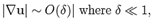 then there is no need for distinguishing between the reference and the current configuration for that body.
3. Axial-symmetric models
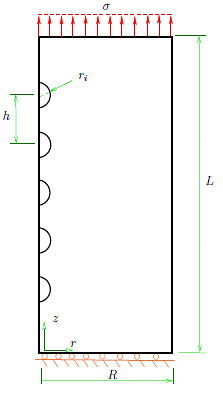
For simplicity, the hyper-elastic matrix is considered to be a cylinder of radius R and length L (see, for example, Figure 1). For a cylinder with one inclusion, it is assumed that the inclusion is located in the center of the cylinder, and that the radius of that spherical body is ri (see Figure 1). It is assumed that there is axial symmetry, therefore, we study a plane problem using the coordinates r and z (radial and axial axis, respectively).
The center of the sphere is located at z = L/2. On the surface z = L we apply a uniform axial load σ. On the surface z = 0 we assume that the cylinder cannot move in the axial direction, but it is free to expand in the radial direction, i.e., uz(r, 0) = 0. On the surface r = R we assume that the cylinder is free. Finally, the spherical inclusion is assumed to be perfectly bonded to the the surrounding hyper-elastic cylinder, i.e., the displacement field is continuous across the surface of the inclusion.
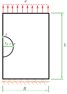
In Figure 2, an hyper-elastic cylinder with two inclusions is depicted.
These two inclusions are of the same radius, are separated by a distance h between centers (the central point between them is located in the middle of the cylinder in the axial line defining it.) The two inclusions are assumed to behave as nonlinear elastic bodies using (10). The rest of the boundary conditions for the problem are the same as the problem presented in Figure 1.
In Figure 3, the case of an hyper-elastic cylinder with five inclusions in a row is presented.
The inclusions are separated to each other by the same distance h. As in the previous case, they are modelled using (10), and the center point for all the inclusions is located in the center of the cylinder.
For the different models mentioned previously, it was assumed that ri = 1 mm. Regarding R, L and h, different cases were considered as indicated in Tables 2-4.
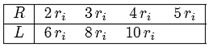
For the case of a cylinder with two inclusions, we assume R = 5ri and L = 10ri (the parameter h is presented in Chart 3.)

Finally, for the case of a cylinder with five inclusions, we assume R = 5 ri and L = 4(h + ), and for h we have the cases presented in Chart 4.

The boundary value problems were solved using the finite element method with an in-house finite element code (details of the method in which the code is based can be found, for example, in Ref. [16].)
4. Numerical results
4.1. Results for one inclusion
In this section we show some results for a cylinder with one spherical inclusion located on its center (see Figure 1), for the cases indicated in Table 2.
In Figure 4, results are presented for the axial and radial components of the normalized stress and the components of the strain, for different values for R, for the case L = 10 ri.
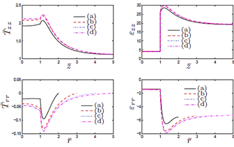
Figure 4. Results for the normalized components of the stress Tzz and strain εzz, for the line r = 0, 0 ≤ z ≤ L/2,and the component Trr of the stress and εrr of the strain,for the line z = 0, 0 ≤ r ≤ R. This is for the case L = 10 ri, where: (a) R = 2 ri (b) R = 3 ri (c) R = 4 ri (d) R = 5 ri.
The normalized components of the stress that appear in Figure 4 are defined as.
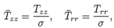
Where σ is the uniform load applied on the upper surface of the cylinder (see Figure 1). The strains are in %. The results for the axial components of the normalized stress and strain Tzz and εzz presented in Figure 4, respectively, are shown for the line  where
where

The results for the radial components of the normalized stress and strain  presented in Figure 4, respectively, are shown for the line
  , where.
In Figure 5 we show similar results as in Figure 4, for R = 5ri and different cases for L.
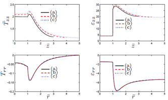
Figure 5. Results for the normalized components of thestress Tzz and strain εzz, for the line , and the component Trr of the stress and εrr of the strain,for the line z = 0, 0 ≤ r ≤ R . This is for the case R = 5 ri,where (a) L = 6 ri (b) L = 8 ri (c) L = 10 ri.
The results for  are shown for the line r = 0,
  while for
  the results are shown for the line
In both Figures 4 and 5 the inclusion is located in the región  and due to the symmetry of the problem, only the upper half part of the inclusion and the cylinder is considered (see Figure 1).
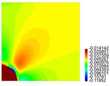
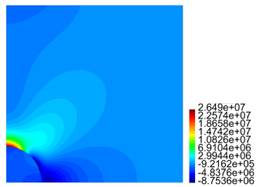
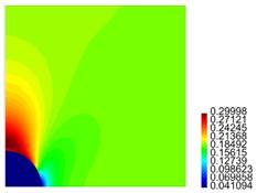
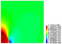
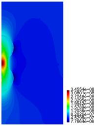
In Figures 6-9 we show results for the radial and axial components of the strain and the stress, for the case R = 5ri , L = 10ri . The stresses are presented in Pa.
4.2. Results for two inclusions
Figure 10 depicts results for the axial and radial components of the stress (normalized stresses, see (18)) and the strain, for the line 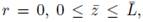 for different values for h as presented in Chart 3 for a hyperelastic cylinder with two inclusions (see Figure 2).
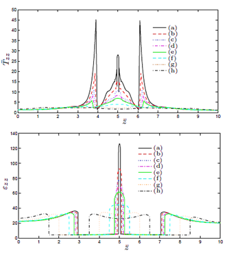
Figure 10. Results for the normalized components of thestress Tzz and strain εzz, for the line r = 0, 0 ≤ z ≤ L,where (a) h = 2.1 ri (b) h = 2.2 ri (c) h = 2.3 ri (d)h = 2.4 ri (e) h = 2.5 ri (f) h = 3 ri (g) h = 4 ri (h)h = 5 ri.
In Figures 11-14 we present results for the radial and axial components of the strain and the stress, for the case h = 2.5 (the stresses are in Pa.)

4.3. Results for five inclusions
Figure 15 presents results for the axial and radial components of the stress (normalized stresses, see (18)) and the strain, for the line 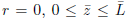 for a hyperelastic cylinder with five inclusions (see Figure 3).

Figure 15. Results for the normalized components of thestress Tzz and strain εzz, for the line r = 0, 0 ≤ z ≤ L,where (a) h = 2.1 ri (b) h = 2.2 ri (c) h = 2.3 ri (d)h = 2.4 ri (e) h = 2.5 ri (f) h = 3 ri (g) h = 4 ri (h)h = 5 ri (i) h = 6 ri (j) h = 7 ri.
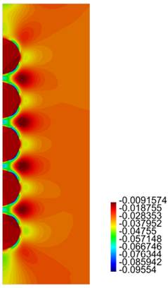
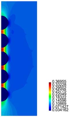
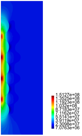
In Figures 16-19 we present results for the radial and axial components of the strain and the stress, for the case h = 2.5ri (the stresses are in Pa.)
4.4. Discussion of the results
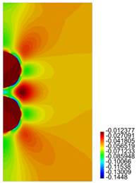
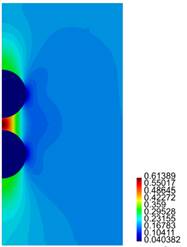
For the matrix with one particle, from Figure 4 cases c) and (d), it is observed there is no meaningful difference between the behaviour of the stress and the strain, i.e., as expected for R large enough, the results tend to be invariant of the size of the cylinder. For the results presented in Figure 5, as in the previous case, for L large enough, there is no much difference in the behaviour of the body. From Figures 4 and 5, we observe that the component of the stress are continuous across the surface of the inclusion, but the components of the strain are not. In both cases, it is recognized the presence of large stresses in the matrix material near the interface with the inclusion, and for Tzz such stresses are positive, which could eventually lead to debonding of the composite. In fact, in Figure 7 we recognize that there is a zone on the upper part of the spherical inclusion (in the matrix), where the radial stress Trr is positive, and that effect is much stronger in the same zone for Tzz (see Figure 9).
For the cylinder with two spherical inclusions, from Figure 10 we observe that there is a considerable difference in the behaviour of the composite if h is varied. Compare for instance the results presented in cases (a), (b) and (d) of that figure, where h = 2.1 ri, h = 2.2 ri and h = 2.3 ri, respectively. The difference in behaviour between Tzz and "zz is large (in particular for the case (a) for Tzz.) In the plot for "zz, we observe the jump in the value for that component of the strain across the interface between the inclusion and the surrounding matrix. In Figures 12, 14 we notice the large values for Trr and Tzz in the matrix, for the zone connecting the two inclusions.
Finally, for the cylinder with five inclusions, as in the previous case, from Figure 15 we notice large values for "zz for the matrix material between the inclusions. Also large values and rapid variations for Tzz in the same zone are observed, especially for the cases (a), (b) and (c). From Figures 16-19 we observe the same large values for the components of the stress and the strain in the zone near the inclusions.
5. Concluding remarks
In the present communication, we have studied the behaviour of a composite consisting of a hyper-elastic matrix with one, two and five spherical inclusions that are modelled using some relatively new classes of constitutive equations, in which, as a particular case such inclusions undergo small strains independently of the magnitude of the stresses. In several of the previous works discussed in the introduction section (see, for example, Refs. [10, 17] and the reference mentioned therein), the main idea of studying constitutive equations of the type (10), (13), was to analyse the behaviour of the solutions for problems exhibiting concentration of stresses, where from the physical point of view, it is expected that the strain remain small. This is the case of brittle bodies with cracks (see the discussion in Ref. [14]). In the present work, this has been also the purpose. Herein, problems exhibiting concentration of stresses near the boundary of inclusions were studied. From the results presented in Section 4, it is observed that indeed there exists concentration of stresses, but strains remain small inside the inclusions. The results presented in this paper should be considered as the outcome of a new way to study the problem of modelling the behaviour of composite materials, where there is a soft matrix filled with a relatively stiff and brittle inclusions.

