


 English (pdf)
 Article in xml format
 Article references
 Send this article by e-mail
 Cited by SciELO
  Similars in
SciELO
Similars in
SciELO  uBio
uBio 
 Permalink
Introduction
Natural gas has come to occupy a significant place in the global energy scenario, with a continuous growth in demand, situation that represents a great challenge for the optimization of the infrastructure associated to gas transportation and distribution. Traditionally, the first stage of a gas transportation project begins with an economic evaluation that, from a technical point of view, uses a steady-state flow analysis to determine the system states parameters. As soon as this evaluation shows the project’s economic feasibility, the design stage of the gas pipeline network begins. It is at this stage that the transient flow analysis is fundamental to the process simulation, in order to adjust the system to real operative conditions and to obtain the highest level of efficiency, compliance and reliability. The large investments associated with the costs of acquisition and installation of gas pipelines and compression stations requires an optimization study of the transportation system, which must be designed to operate under different gas-consuming scenarios, such as the load increase in peak hours, gas pipeline fractures facility maintenance, among others. The simulation of natural gas pipelines and networks requires mathematical models that describe flow properties. Some models that have been developed year after year based on the laws of fluid mechanics that govern this process, interpreted as a system of equations difficult to solve. Several iterative methods have been implemented for their resolution, using at the same time, different schemes of discretization and restrictive assumptions. There are various works related to the simulation of transient flow in gas pipelines, among which is the method of characteristics (MC). This method takes the partial differential equations system and transforms it into ordinary derivatives to then be numerically integrated. An advantage of the method is that it can handle discontinuities in the simulation, although the main disadvantage is that it is comparatively slow; the time steps must be small enough to satisfy the Courant-Friedrichs-Lewy Condition (CFL) (Issa & Spalding, 1972; Wylie & Streeter, 1978).
The Crank-Nicolson method (CNM) for isothermal gas flow, solve the continuity and momentum equations, node to node, applying a discretization scheme of finite differences (Guy, 1967; Heath & Blunt,1969). The main disadvantage of this method is that it not always gives a stable solution according to the Von Neumann stability analysis for large time steps. The finite differences method (FDM) for isothermal flow in gas pipelines and networks (Kiuchi, 1994), integrates the system of equations in partial derivatives, using a totally implicit discretization scheme with some simplifications. After neglecting the convective term in the moment equation, the Von Neumann stability analysis showed that the discretized equations are unconditionally stable. In a later study, the FDM for non-isothermal flow is applied (Abbaspour & Chapman, 2008), this time incorporating the convective term in the momentum equation, treating the compressibility factor as a function of temperature and pressure and considering the friction factor as a function of Reynold’s Number and of the pipe roughness. On the other hand, Patankar (1980) presents the finite volume method (FVM), an alternative to represent and evaluate partial differential equations in the form of algebraic equations, expressing the principles of conservation of the underlying physics in forms of macroscopic balance of a specific property. Versteeg and Malalasekera (2007) indicate that integration of the control volume is what distinguishes FVM from other computational fluid dynamics (CFD) techniques. A relation between the numeric algorithm and the principles of mass conservation (continuity), momentum and energy, constitutes one of the main attractions of this approach and makes its concepts much easier to be understood by engineers. This research work consists in describing a simplified mathematical model, discretized with FVM, that allows computational simulation of gas flow transport for different entry and exit conditions, considering transient regime and that the fluid is transmitted in gas pipelines. The model is validated through comparison with known models.
Methodology
1. Constitutive equations
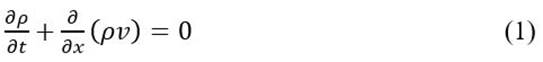
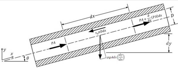
Issa and Spalding (1972), Van Deen and Reintsema (1983) and Thorley and Tiley (1987) develop equations 1-5, where they describe the properties of compressible single-phase one-dimensional flow, over a control volume of constant surfaces, framed within a gas pipeline (Figure 1). These equations are governed by fluid dynamics principles, they include the effects of wall friction and heat transfer and are position and time-dependent.
Continuity equation:
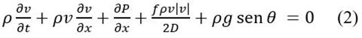
Momentum equation:
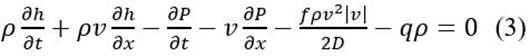
Energy equation:
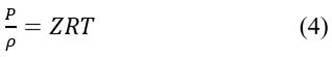
State equation:
Wave propagation velocity:

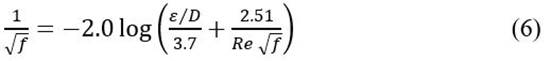
The friction factor f is calculated with Reynold’s Number Re and the gas pipeline roughness ε/D with Colebrook equation 6, which combines flow regimes both partial and totally turbulent and is the most suitable for cases where the pipeline is operating in the transition zone (Mohitpour, Golshan & Murray, 2003).
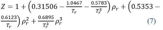
The compressibility factor Z is obtained from equation 7 (Dranchuck, Purvis & Robinson, 1973).
2. Simplification
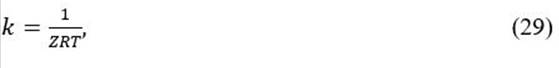
By considering that the flow is isothermal, it is assumed that temperature changes in the fluid are slow enough to be canceled by heat conduction and the environment that surrounds it; in consequence, the energy equation is neglected and the system is now conformed by the continuity equation 8, the momentum equation 9 and an approximate relation (equation 10), between the state equations and wave propagation velocity (Kiuchi, 1994).


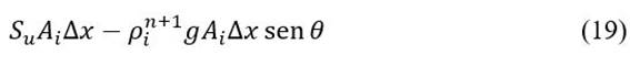
In equation 9, the first two terms are inertial: the first one is transient, the second one is convective; the third one is the pressure drop; the fourth is the source term, and the fifth one is the gravity term. The Z factor in natural gas, for pressure and temperature ranges from 0.5 MPa to 6.5 MPa and from 280 K to 320 K. In both cases, this factor oscillates between 0.8 and 1.0, approximately. In addition, the values of the partial derivatives of Z with respect to pressure and temperature are negligible.
3. Discretization scheme
The FVM contains discretization schemes for the key treatment of transport phenomena, convection (transport due to fluid flow) and diffusion (transport due to variations in the variable from node to node), as well as the source terms (associated to the creation or destruction of the variable) and transient (variable variations with time).
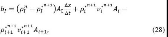
In the discretization mesh (Figure 2) the node I has as neighbors the nodes I −1(to the left) and I + 1(to the right). Between the nodes I −1 and I, is the surface I that corresponds to the left face of the control volume constructed around I. Between the nodes I and I + 1, is the surface I + 1that corresponds to the right face of the considered control volume. The distances between the surfaces (faces) and between the nodes (centers) are ∆x. As the flow model geometry is one-dimensional, the control volume is calculated by V = A ∆x.
Continuity equation: The velocities are located in their respective surface and the density, in the node or control volume center (Figure 2).


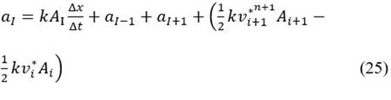
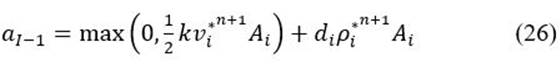
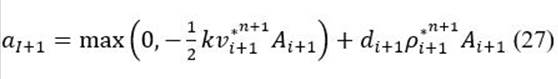
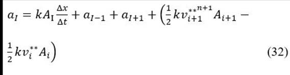
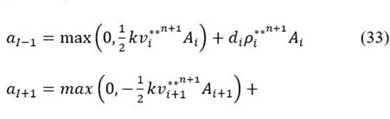
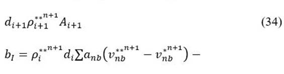
Momentum equation: The control volume is delayed in the mesh at a distance of ½ ∆x from node I (Figure 3), so that the pressures coincide in the nodes and the velocities coincide in the surfaces.


It is established that  1is the value of the previous iteration.
If the Upwind (UW) scheme is used, then 
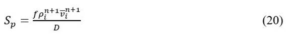
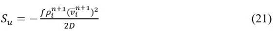
If the Total Variation Diminishing (TVD) scheme is used, then the source term correction is:

With

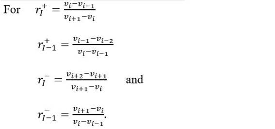
The flow limiting function UMIST is established to prevent the generation of spurious oscillations:

4. Implementation
The FVM implementation consists in following the steps described in the algorithm 1, for a space-time domain of N control volumes and t = 0, t + ∆t, . . . , tmax seconds; calculating for these volumes and seconds (Figure 2) the pressure fields located in the nodes or centers (I) and velocities in the surfaces or faces (i),in the present time levels (n + 1), by means of the Tridiagonal Matrix Algorithm (TDMA) for coupled systems of prediction-correction based on the constitutive flow equations and adapted to initial conditions in the present time level (n) and boundary conditions in the natural gas pipeline’s entry (i = 1) or exit (i = N + 1).
Require: Tgas, Po, vo, D, L, θ, f, tmax, ∆t, N
Ensure: P, ρ, v
Step 1: Establish: 𝑡 = 0, 𝑛 = 0
Step 2: Calculate the compressibility factor Z
Step 3: Calculate initial density 𝜌𝑜
Step 4: Calculate initial conditions for stable flow: 𝑃𝑛, 𝜌𝑛, 𝑣𝑛
Step 5: Calculate boundary conditions for the time 𝑡 + Δ𝑡:

Step 6: Establish:
Step 7: Apply the Semi-Implicit Method for Pressure Linked Equations (SIMPLE) or the Pressure Implicit with Splitting Operators (PISO) iterative algorithm until convergence.
Step 8: If t < tmax, then establish:
𝑡 = 𝑡 + Δ𝑡
𝑛 = 𝑛 + 1
return to step 5.
End If
Patankar (1980) proposes an algorithm named with the acronym SIMPLE. The procedure consists in systematically estimating and correcting velocities and pressures on an alternated mesh (algorithm 2). The discretized continuity (equation 11) is rewritten as a connection equation for pressure, that is:

Where:

Require: 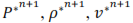 (initial condicions).
Ensure: 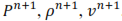
Step 1: Solve the discretized momentum equation:

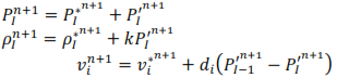
Step 2: Solve the correction equation for pressure:

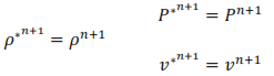
Step 3: Correct pressure, density and flow velocity:
Step 4: If it does not converge, then establish:
return to step 1.
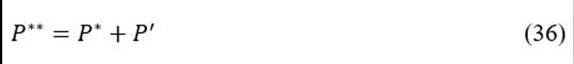
Another calculation procedure of pressure-velocity named with the acronym PISO was originally developed by Issa (1986) and presented by Versteeg and Malalsekera (2007) for the iterative calculation of compressible flow. The PISO algorithm implies one predictive step and two correcting steps (Figure 6) and it can be seen as an extension of SIMPLE with one additional corrective step to improve it. Thus, the second correction equation is established as:

Where:


Considering now that:


Algorithm 3 PISO
Require:  (initial conditions).
Ensure: 
Step 1: Solve the discretized momentum equation: (SIMPLE).

Step 2: Solve the first correction equation for pressure:(SIMPLE).

Step 3: Solve the second correction equation for pressure:

Step 4: Correct pressure, density and flow velocity:

Step 5: If it does not converge, then establish:
return to step 1.
End If
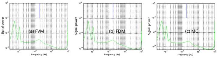
In order to obtain a convergence behavior indicator through the whole flow field, the global residue R v is defined as the sum of local residues over all the control volumes domain (N), that is:
Results
Based on the comparison of flow simulations, two evaluations were made for a gas pipeline in horizontal position of 5 km length and 50 cm inner diameter. The fluid is natural gas, the operation temperature is 25° C and the input pressure is set at 5 MPa. The gas pipeline ́s natural frequency is 0.0179 Hz, calculated by means of the relation ωn= c/4L (Kiuchi, 1994). It initiates under flow conditions of steady-state. The Darcy-Weisbach friction factor is considered constant and equal to 0. 008.All the simulations were made with Scilab compiler, running the algorithms for FDM and MC. Simulations and the FVM were made under two implementation modalities: one applies the UW scheme in conjunction with the SIMPLE algorithm, while the other one uses the TVD-UMIST scheme with the PISO algorithm.
The proposed model and the reference models, were simulated for different sizes of space-time step, specifically test runs were done with time steps (∆t) of 1/10, 1and 10 s, section numbers or control volumes (N)of10, 50 and 100, obtaining very good results for the models based in FVM and FDM, which was not the case working with MC, due to the stability condition CFL. With the purpose of preserving the iterative process stability for all the models, simulations with ∆t = 1s y N = 10, are shown in Figure 4
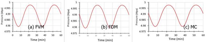
1. Evaluation 1: Relatively slow transient flow
His evaluation model is taken from Vieira and Torres-Monzón (2013) and Yow (1971), and it consists in the sinusoidal mass flow variation at the gas pipeline exit; it initiates with 20 kg/s in stable state; the flow variation amplitude is 10 kg/s and the oscillation period is 1800s. In figures 5 to 8, the FVM gives nearly equal results as FDM, both for the mass flow and pressure along the gas pipeline, showing the same oscillation frequencies in each spectral signal. Comparison between FVM and MC gives similar values in the calculation of flow properties and the spectral analysis shows a slight phase shift.

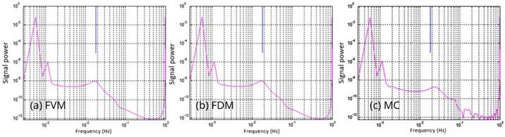
Fig. 6 Spectral analysis for the wave signal generated by the mass flow at the natural gas pipeline entry compared with the natural frequency ωn(blue line).
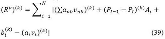
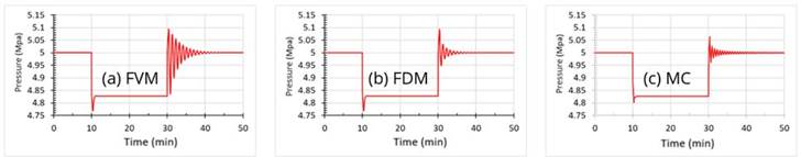
2. Evaluation 2: Fast transient flow
Abbaspour and Chapman (2008) and Kiuchi (1994) propose as an evaluation model, the valve’s opening and closure at the gas pipeline exit section. The valve opens after ten minutes, the mass flow increases from 0 to 80 kg/s and after twenty minutes in the same conditions, the valve completely closes. In figures 9 to 12, FVM agreed with FDM for mass flow and pressure, before and after opening but they disagreed after total closure for some minutes, both oscillated with the same frequencies, FVM showing bigger amplitude than FDM; this is primarily due to that the alternative model considers the convective term in the iterative process, while the other model neglects this term. In the spectral analysis, after the exit valve is closed, both signals tend to a peak and coincide with the natural frequency, fact that indicates the presence of resonance in the gas pipeline. On the other hand, if FVM is compared with MC, both show differences, especially after total closure, although both models ended up converging in minutes. The oscillations differed in amplitudes and frequencies, the spectral analysis of MC showing a phase shift between the peak and the natural frequency.
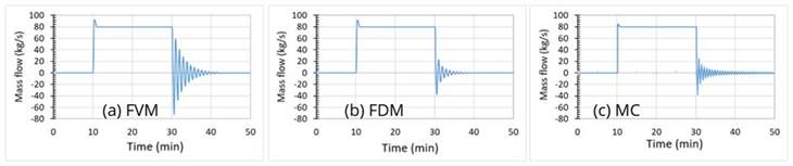
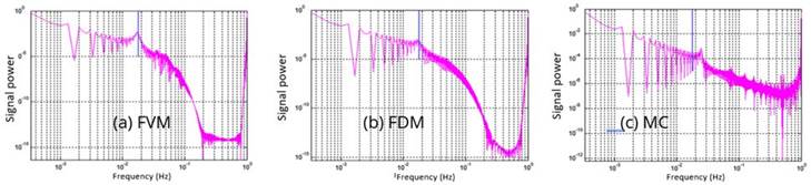
Fig. 10 Spectral analysis for the wave signal generated by the mass flow at the natural gas pipeline entry compared with the natural frequency ωn (blue line)

Conclusions
The transient flow model based in FDM and FVM with two modalities: UW with SIMPLE and TVD-UMIST with PISO, subjected to transient flow problems for a wide range of space-time step sizes. Both resulted stable models and more tolerable to the CFL condition. The convective term of the momentum equation plays an important role in the gas flow calculation and it is not discarded for the FVM, because this term’s effect is more significant when the flow rate decreases abruptly in the gas pipeline. Finally, taking as reference the previous exposition, the proposed model based on FVM turns out to be a reliable alternative for the calculation of isothermal flow in gas pipelines with an efficient response to slow and fast oscillations.

