


 Inglés (pdf)
 Articulo en XML
 Referencias del artículo
 Enviar articulo por email
 Citado por SciELO
  Similares en
SciELO
Similares en
SciELO 
 Permalink
1. Introduction
Modeling and simulation of heat exchangers are essential for continuous improvement and control of productive processes. They are considered as effective engineering tools, usually applied to the study, upgrade and optimization of different industrial systems (Toro-Carvajal, 2013; Ferreira, Nogueira & Secchi, 2019). Despite the diverse principles that are utilized to classify these models nowadays, they can be broadly categorized into two major groups: [1] those depending on the overall heat transfer coefficient, and [2] alternative models that eludes calculation of the overall heat transfer coefficient.
A vast amount of works is available on the first group. While some authors performed mathematical modelling of shell-and-tube heat exchangers (Turgut, Turgut & Coban, 2014; Markowski & Trzcinski, 2019; Sánchez-Escalona & Góngora-Leyva, 2019) and triple concentric-tube heat exchangers (Batmaz & Sandeep, 2005; Patrascioiu & Radulescu, 2015; Radulescu, Negoita & Onutu, 2019), there are other studies related to numerical modelling of these equipment (Rao & Raju, 2016; Bayram & Sevilgen, 2017; Taler, 2019; Xavier-Andrade, Quitiaquez-Sarzosa & Fernando-Toapanta, 2020). In spite of its broader application, the overall heat transfer coefficient entails time-consuming calculations as well as using heat transfer correlations that regularly provides inaccurate results, with errors ranging up to 40 % (Laskowski, 2011; Markowski & Trzcinski, 2019).
The second group of investigations is mostly comprised by “black-box” solutions and dimensional models. As part of the former, the use of Artificial Neural Networks on this field is extensive, but encloses the following shortcomings: it is difficult to obtain the model explicit equations; there is scarce information about the influence of independent variables on the responses; and mandatory use of a computer or scientific calculator to evaluate the resultant equation (Mohanraj, Jayaraj & Muraleedharan, 2015; Mohanty, 2017; Sánchez-Escalona &Góngora-Leyva, 2018). On the other side, although the dimensional modeling overcomes previous drawbacks, just a few researchers has concentrated on simulating heat exchangers. Laskowski (2011, 2012) proposed model equations for prediction of discharge temperatures in two high-pressure regenerators, which were installed in a 200 MW power plant. He later studied a steam condenser, in order to present succinct and approximated heat-transfer effectiveness expressions. Afterward, Sánchez-Escalona, Góngora-Leyva & Camaraza-Medina (2019) stablished a model for output predictions on a monoethanolamine heat exchangers system. However, none of the authors utilized the Buckingham Pi-theorem for performance anticipation on three-fluid heat exchangers.
Considering this gap, current contribution investigated the application of dimensional analysis to modeling and simulation of jacketed shell and tube heat exchangers (JS&THE). Since an operational set of hydrogen sulphide gas coolers was evaluated, the model would facilitate quick anticipation of the equipment performance, besides straight-forward assessment of different plant operational scenarios.
2. Materials and methods
2.1. Applied methodology
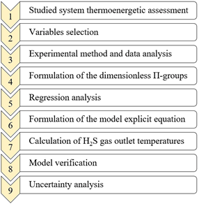
This research first focused on identifying parameters with a remarkable influence on three-fluid heat exchangers performance. Next, the experimental method was utilized to collect the data sets of explanatory variables. The non-dimensional groups were subsequently obtained, followed by resolution of the explicit functional from by applying a multivariate regression analysis. Lastly, the model confirmation was performed by comparing computed results versus measured hydrogen sulphide discharge temperatures. The methodology steps are detailed below (Figure 1).
The statistical parameters utilized to validate the model were: correlation coefficient, Nash-Sutcliffe index, as well as absolute errors (or bias errors) and percentage errors (Ekici & Teke, 2018; Li & Lu, 2018; Pérez-Pirela & García-Sandoval, 2018). The uncertainty analysis was grounded on the Law for the Propagation of Uncertainty, in a case where input quantities are not correlated. It is based on an approximation of first-order of the Taylor series, assuming a symmetrical distribution probability of the errors. In single-sample experiments, where studied variables can not be recurrently measured under the same conditions, uncertainty within the results is evaluated from the systematic errors introduced by direct experimental readings, in preference to statistical analysis of a sequence of experimental observations (JCGM, 2008; Uhia, Campo & Fernández-Seara, 2013).
2.2. System description
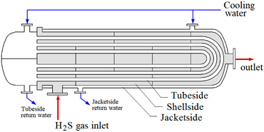
This research examined a system of hydrogen sulphide gas coolers that is online, located on facility which produces 99.8 % pure hydrogen. Installed equipment are three-fluid heat exchangers, shell and tube type, having the designation “BEU with external jacket” according to TEMA (2019). Its main function is cooling down the hydrogen sulphide stream from 416.2 to 310.2 K. Construction materials were stainless steel, 316L AISI-grade. Additional design parameters are listed on Table 1. Inside the equipment, the gas flows through the shell, in a unique pass, while the coolant circulates at the tubeside and the external jacket, in four passes and single pass, respectively. Since cooling water is fed from a common pipe header, the tubeside and the jacketside inlet temperatures were assumed the same (Figure 2).

2.3. Variables selection
The equations of heat transfer pertained to heat exchangers were used as starting point for selection of the model variables. Equation 1 was derived from the first law of thermodynamics, while Equation 2 was obtained from the ε-NTU method. Note that mentioned expressions are acceptable for monophasic streams, steady flow and steady state, as well as negligible heat losses leaking to the surroundings. Additionally, it was assumed that the overall heat transfer coefficients, the specific heat of the fluids, and other thermo-physical properties remain invariant across the heat exchangers (Nitsche & Gbadamosi, 2016).
(1)
(2)
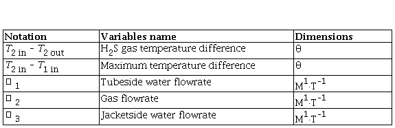
Where: Cp – specific heat at constant pressure, J/(kg·K); ɛ – heat exchanger heat transfer effectiveness; . – heat transfer rate, W; . – mass flowrate, kg/s; Δ. – temperature difference, K;
– maximum temperature difference between the hotter and the colder fluid.
Previous equations were related by means of a heat and mass balance applied to JS&THE, as stated in Equations 3 and 4:
(3)
(4)
The subscripts are: 1 – tubeside water; 2 – hydrogen sulphide gas; 3 – jacketside water; . – shellside-to-tubeside thermal communication; II – shellside-to-jacketside thermal communication.
Since both water inlet temperatures are equal, the maximum temperature differences remain the same, i.e.
Hence, Equation 4 was re-written as Equation 5:
(5)
The heat transfer effectiveness, defined as the ratio between current heat transfer rate to the maximum heat exchange rate that is theoretically possible, is also a function of non-dimensional parameters like the heat transfer rate ratio (Cr) and the number of transfer units (NTU), as expressed in Equation 6 (Laskowski & Lewandowski, 2012; Nitsche & Gbadamosi, 2016):
(6)
The heat transfer rate ratio and the number of transfer units are calculated according to Equations 7 and 8:
(7)
(8)
Where: . – heat transfer area, m.; . – overall heat transfer coefficient, W/(m.·K).
At this point, functional relationship amongst dependent and independent variables was defined through Equation 9, which represents an abbreviated form of Equation 5 under the following considerations (Laskowski, 2011; Sánchez-Escalona et al., 2019):
§ constant specific heats,
§ constant fluids thermo-physical properties,
§ invariant heat transfer areas, and
§ overall heat transfer coefficients are function of flowrate and inlet temperature of the fluids.
(9a)
(9b)
Previous equation utilized the temperature differences instead of individual temperatures, as independent variables, in order to simplify the model. Primary dimension for Δ. and . are the same.
2.4. Experimental method
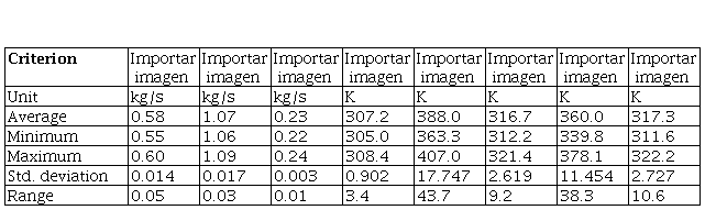
Due to the continuous production philosophy of the plant, the passive experimental method was utilized. It consisted of measuring and observing input and output variables within the usual working regime of researched set of heat exchangers, hence studying the heat transfer phenomenon as it happens (Edmonds & Kennedy, 2017). Readings of mass flowrates, inlet temperatures and outlet temperatures were carried out on all fluids, using the instruments listed in Table 2. The database included 80 data points, which are statistically described in Table 3.
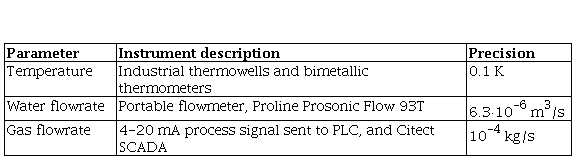
Table 3 Variables descriptive-statistical summaryWhere: T cold in – water inlet temperature, K; T hot in – gas inlet temperature, K; T 1 out – outlet temperature of the tubeside water, K; T 2 out – outlet temperature of the gas, K; T 3 out – outlet temperature of the jacketside water, K.
2.5. Dimensional analysis
In principle, the dimensional analysis is a tool for lessening the quantity and complexity of the experimental variables that describes a physical phenomenon. In this way, experiments which might result in several parameters can be reduced to a single set of curves, or even a unique graph, if properly non-dimensionalized (Zohuri, 2015; Al-Malah, 2017).
There are several methods of reducing a number of dimensional variables into a smaller amount of dimensionless groups. In such ambit, the Pi-theorem enunciated by Buckingham is a key approach. It affirms that the Π (Pi) quantities that remains after completing a dimensional analysis are equivalent to the difference amongst the number of quantities describing the problem and the maximum number of these being dimensionally independent (this last will always be equal to or less than the quantity of fundamental dimensions required to write all dimensional equations). Once obtained, Π-groups are related according to Equation 10, with the exact structure of the functional form being achieved on the basis of experimental data (Ekici & Teke, 2018; Zohuri, 2015).
(10)
Formulation of the dimensionless Π-groups initiated with the method of repeating variables, where the initial step consisted of writing every variable and their primary dimensions (Table 4).
As perceived, five variables ( n=5 ) that involves two independent fundamental physical quantities ( j=2 ) were used to characterize the heat transfer phenomenon taking place within the JS&THE. Hence, three dimensionless groups were projected ( n-j=3 ), as presented from Equation 11 to Equation 13. The repeating variables that were selected are: maximum temperature difference , and hydrogen sulphide gas mass flowrate
(11)
(12)
(13)
Constant exponents . and . were determined by substitution of the variables by their dimensions and making the Π-groups to be non-dimensional, as defined in Equation 14 to Equation 16.
(14)
(15)
(16)
By definition, primary dimensions are independent from each other. Hence, the exponents of each primary dimension were individually zeroed to solve the equations. As a result, p1 = –1, q1 = 0, p2 = 0, q2 = –1, p3 = 0 and q3 = –1. After substitution of computed exponents into the initial equations, the final Π-groups expressions were formulated. They are denoted by Equations 17, 18 and 19:
(17)
(18)
(19)
Then, consistent with the definition given through Equation 10, the model hypothetical formulation was written in the form of Equation 20:
(20)
2.6. Model formulation
Functional relationship between the Π-groups was later determined by using a least-squares multivariate linear regression, hence obtaining a model with the mathematical structure of Equation 21.
(21)
Where b0, b1 and b2 are curve-fitting coefficients. Then, the mathematical function that correlates the above-defined Π-groups took the form of Equation 22:
(22)
Finally, the model explicit equation utilized to calculate the hydrogen sulphide gas outlet temperature was obtained by substitution of Equation 17, 18 and 19 into Equation 22, and convenient rearrangement of the terms:
(23)
3. Results and discussion
3.1. Predictive ability performance
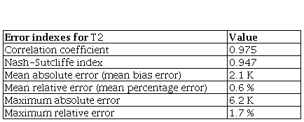
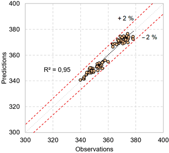
Since computed divergences are slight in the technological process under analysis (Table 5), attained shortcut equation is considered suitable for predicting the heat exchangers performance under varying plant operational conditions. Calculated coefficient of determination informed that 95 % of the output temperature variability was explicated by current model (Figure 3), which is applicable within the following validity ranges: 0.55 ≤ m1 ≤ 0.60, 1.06 ≤ m2 ≤ 1.09, and 0.22 ≤ m3 ≤ 0.24 (units in kg/s).
3.2. Trend analysis
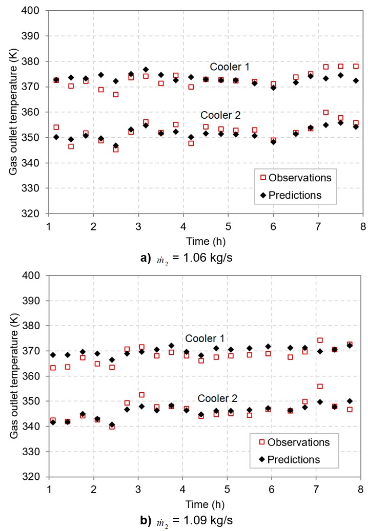
The satisfactory agreement between model predictions and experimental observations is confirmed on the following trend graphs (Figure 4).
As observed, the gas exit temperature rises over time, mainly caused by progressive efficiency losses. They are ascribed to ongoing sulphur buildups around the surfaces of heat transfer, caused by fluid pressure and temperature drops, thus creating isolating layers that lessen heat transfer effectiveness (Sánchez-Escalona & Góngora-Leyva, 2019). On the other hand, since the researched system consists of two identical JS&THE, installed in a series/parallel layout —with the gas flowing in series, and cooling water in parallel—, the hotter shell (cooler 1) provides a greater heat duty as compared to the colder one (cooler 2), essentially because of the higher mean temperature difference. This last fact was better illustrated through a thermographic picture of the facility under analysis (Figure 5). It shows two sets of hydrogen sulphide gas coolers, having the left-hand exchangers operating in the cooling cycle, while the right-hand ones were turned over to the online cleaning stage by using intermediate pressure steam (0.586 MPa average). Regardless the operational cycle, the higher temperatures and greater heat loads were confirmed on the first stage (cooler 1) of each set, i.e. lower-side heat exchangers.
It was also experimentally confirmed that heat exchangers did not reach the envisaged performance under observed exploitation conditions. The gas exit temperature exceeded the design value (310.2 K) farther along in 53.1 K, while the tubeside water flowrate supplied to each exchanger represented from 49.86 to 54.77 % of the targeted flow (1.1 kg/s). Besides, water never made it to the turbulent regime, as expected for optimum heat transfer. Maximum Reynolds number of 2378 and 502 were calculated for tubeside and the jacketside streams, respectively.

Application of depicted mathematical modelling techniques assisted the authors in providing a succinct list of technological solutions and organizational actions that will contribute to improve the heat exchangers efficiency:
§ to reduce the operational time from eight to six hours (after each cooling cycle, online cleaning is performed with steam flowing through the tubes and the jacketside),
§ to perform offline cleaning of the tube-bundle,
§ to increase water flowrates until reaching a turbulent flow,
§ to optimize baffle spacing, considering that a hydrogen sulphide flowrate incremental would result in lower fouling rates and enhanced heat transfer.
3.3. Uncertainty level
When applying the model explicit expression —Equation 23—, the true outlet temperature value for the hydrogen sulphide gas is expected to lie within the band ± 0.637 K, with an embedded 95 % confidence level. It was calculated from Equation 24 and 25, utilized for computation of the expanded uncertainty assuming a normal distribution in the experimental results.
(24)
(25)
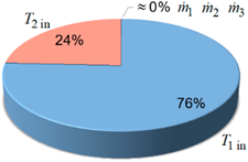
It was observed that the inlet temperatures have the greatest influence on the uncertainty of the results, while a negligible effect was introduced by fluids flowrates (figure 6). Hence, the selection of more accurate temperature-reading instrumentation is essential, if upgraded outputs are entailed.
4. Conclusions
A shortcut model was proposed for predicting hydrogen sulphide gas discharge temperature in JS&THE. In this respect, the dimensional analysis and the Buckingham Pi-theorem were successfully applied. Comparison of predicted values versus experimental readings resulted in a correlation coefficient of 0.975, and a Nash-Sutcliffe index of 0.947. The mean absolute error was 2.1 K, while deviations (percentage errors) did not exceed 1.7 %. Calculated expanded uncertainty was as low as ± 0.637 K.
On this research the attained explicit equation provided reliable results, and it is of a simpler use for determining the main fluid exit temperature if compared to methods like the ɛ-NTU, that relies on computation of the overall heat transfer coefficient. Major shortcoming consist of the limited application of Equation 23, since not recommended for heat exchangers modeling other than the studied set, nor input variable values outside declared validity ranges. However, this research outcomes are of importance in the assessment of the heat exchangers performance and, consequently, in the improved operation of related industrial process.
Future works are focused on curve-fitting over a wider range of experimental data, in order to extend the model boundaries, as well as performing symbolic regression to obtain alternative mathematical functions that better correlates the dimensionless Π-groups.

