


 Inglés (pdf)
 Articulo en XML
 Referencias del artículo
 Enviar articulo por email
 Citado por SciELO
  Similares en
SciELO
Similares en
SciELO 
 Permalink
1. Introduction
State estimation is an important topic which contributes to the proper management of electrical energy. In this sense, fields where the application of state estimation methods is crucial such as modeling, optimizing power flow, bad data detection, contingencies analysis and corrective actions against possible failures in the power systems improve the monitoring capability of the grid to take control actions in real-time raising the system reliability and stability, (Huang et al., 2012). State estimation is mainly used in the tracking of the dynamics of the power system through the assimilation of real-world information obtained from smart measurement devices.
The Static State Estimation provides the system operating point in a determined time reflected through the state variables for each measurement data set and has no memory of the evolution of the state variables, it was introduced by Schweppe and Wildes (1970), based on Weighted Least Square (WLS). Dynamic State Estimation (DSE) was also introduced by Debs and Larson (1970) with a simple model for the time behavior of the power system.
Kalman filters are widely used for the analysis of dynamic systems with normally distributed noise: the EKF applied for non-linear systems, the unscented Kalman filter, and the ensemble Kalman filter; researchers are also studying the particle filter and other stochastic methods.
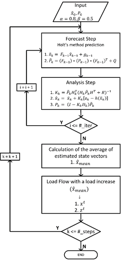
In this work, the performance of the EKF focused on forecasting and filtering the state vectors by using exponential smoothing and recursive Bayesian estimation in the state estimation process of the EPS (see Figures 1and2) can predict state vectors one-time step ahead based on the priori knowledge (prediction stage) and be corrected (update stage) with next measurement sets. The dynamics of the system is simulated using smooth load changes. The loads were changed in each time step with a linear tendency, and the method of Holt has been used to linearize the state transition.
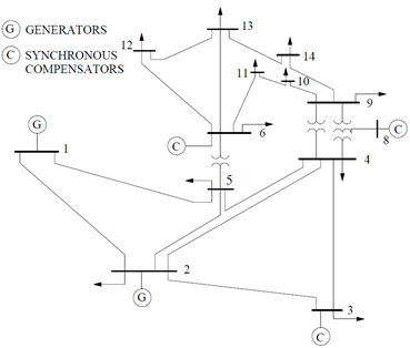
The electrical power systems with their data considered in the study are the IEEE 14 and 30 bus test cases, which represent a portion of the American Electric Power System (in the Midwestern US) as of February 1962. These and others IEEE n-bus test cases are used as a reference for different studies, and they are found in the archives of the University of Washington (Washington, 1993).

The extended Kalman filter consists of the linearization of the nonlinear system about a nominal state trajectory and the posterior approximation of the probability density function (pdf) as Gaussian.
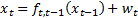
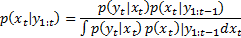
The nonlinear system in Equations 1 and 2 is considered in the derivation of the EKF by using the Recursive Bayesian Estimation approach,
 (1)
(1)
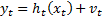 (2)
(2)
with  the non-linear function relating the state propagation through time and
  the non-linear observation function. The distributions and statistics of the process and observation noises are presented as shown in Equations 3 - 8.
 (3)
(3)
 (4)
(4)
 (5)
(5)
 (6)
(6)
 (7)
(7)
 (8)
(8)
The noises are white Gaussian distributed with zero mean and uncorrelated  with
with  ,
,  and
and  are positive definite covariances matrices for the process and observation noises respectively, and
  is a positive integer.
Based on the fact that the nonlinear system is linearized before the analysis step, the posterior pdf at time step  can be approximated by the Gaussian distribution in Equation 9,
 (9)
(9)
where  is the true state vector,
  and
and  are the state vector and the covariance matrix, obtained both from the analysis step at time step
  .
.
Forecast step . The forecast step is given by the computation of the predictive pdf in Equation 10.
 (10)
(10)
The posterior pdf at time is referred in Equation 9. The transition pdf at the right hand side of Equation 10 can be obtained from Equation 1 and by considering that this pdf follows the Gaussian distribution in Equation 11;
 (11)
(11)
thus, the predictive pdf is defined as in Equation 12.
 (12)
(12)
The integral in Equation 12 is complicated due to the presence of the nonlinear function  (
( ).
).
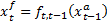
The approach adopted in the extended Kalman Filter is the linearization by using Taylor series. Additionally, a state trajectory should be defined around which the function is linearized. At this point in the development of the extended Kalman Filter, the best estimate is given by .
Taylor series expansion of  in a neighborhood of
  is considered in the linearization of the system. For the linear approximation, only the first two terms are considered.
The resulting prior pdf can be obtained in the Gaussian form as in Equation 13.
 (13)
(13)
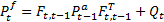
The forecast state vector  and forecast error covariance matrix
  are given by Equations 14 and 15.
 (14)
(14)
 (15)
(15)
Analysis step . The analysis step consists in the update of the prior according to Equation 16.
 (16)
(16)
For the extended Kalman filter, the prior is approximated by a Gaussian distribution which is characterized by the mean (Equation 14) and the covariance (Equation 15). The likelihood pdf is obtained from Equation 2, by considering that the pdf in Equation 17 is Gaussian.
 (17)
(17)
By substituting Equation 13 and Equation 17 into Equation 16, the filtering pdf is given by Equation 18,
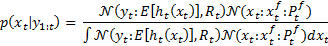 (18)
(18)
where the first issue aiming to calculate the filtering pdf is to solve the integral in the denominator. In order to find an analytical solution, the observation system is linearized around a state trajectory. At this point,  is the best state estimation thus the nonlinear observation system is linearized through Taylor series expansion in the neighborhood of . The non-linear function is expanded as in Equation 19,
 (19)
(19)
where  is a
is a  dimensional Jacobian matrix.
By substituting Equation 19 into Equation 18, the expression for the posterior pdf is given in Equation 20.
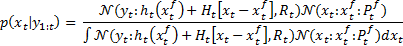 (20)
(20)
Now, the solution of the integral is tractable, and the resulting expression for the posterior pdf in terms of distribution is (Equation 21):
 (21)
(21)
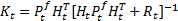
with (Equations 22 and 23)
 (22)
(22)
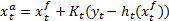
and Equation 24.
 (23)
(23)
 (24)
(24)
The algorithm for the extended Kalman filter is described in Algorithm 1.
For  to the number of time steps
Forecast step:
2. Analysis step:

2. Methodology
The Electrical Power System
To simulate the slow dynamics of the test systems under normal conditions, the smooth load changes were obtained by running load flow calculations under different loading conditions at each step (Valverde and Terzija, 2011). The dynamics of the system was obtained by varying the loads at certain predefined buses (4, 5, 7, 9-14 for the 14- bus system and 3, 4, 6, 7, 9, 10, 12, 14-30 for the 30- bus system) following a linear trend of 1% over the entire time interval with a random fluctuation of 3%. Additionally, measurements of voltage, power injections, and power transfer were corrupted with a random additive Gaussian distributed noise with a mean equal to zero and a low level of variability, this is, with a standard deviation (σ) according to Table 1 (Sharma, Srivastava, and Chakrabarti, 2017) for voltage and powers respectively, to consider the uncertainty of measurement.
Table 1. Values of standard deviation Measurement 
| Power Injection in pu. | 0.001 |
| Power Flow in pu. | 0.001 |
| Voltage in pu. | 0.0006 |
| Angle in rad. | 0.018 |
The state variables were the voltage  and angle
  magnitudes of each one of the bars. Bus 1, in both systems, was considered the slack bus with angle 0°. Buses 1, 2, 3, 6, 9 for the 14-bus system and buses 1, 2, 5, 8, 11, 13 for the 30-bus system were buses with a regulated voltage. The 14-bus system had 73 measurements, from which 5 were voltage magnitudes, and the rest were power magnitudes. The 30-bus system had 93 measurements, from which all were power magnitudes except the first that was a voltage magnitude.
Performance indices
The accuracy of EKF are carried out using the following indices as seen in previous studies (Alhalali and Elshatshat, 2015; Valverde and Terzija, 2011):
(1) The error estimation ε(k) for step k (Equation 25):
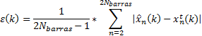 (25)
(25)
(2) The error estimation ε(n) for bus n:
 for voltage magnitude (Equation 26):
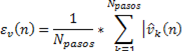 **
**
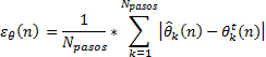
 for angle magnitude (Equation 27):
 (27)
(27)
 (28)
(28)
where,  is the state vector
 ,
,  is the mean error for the
  ,
,  is the filtered (estimated) state vector at step and
  bus,
bus,  is the number of buses,
  is the mean error for the bus, is the error estimation calculated for voltage magnitude at bus,
  is the filtered (estimated) voltage magnitude at bus and step,
  is the true (actual) voltage magnitude at bus and step, is the error estimation calculated for angle magnitude at bus,
  is the filtered (estimated) angle magnitude at and step,
  is the true (actual) angle magnitude at and step,
  is the number of time steps (sampling time),
  is the calculated performance index for step ,
  is the number of measurements (observations),
  is the estimated measurement vector at
  measurement and step,
  the real measurement vector at measurement and step,
  is the true measurement vector at measurement and step.
Extended Kalman Filter - EKF
The non-linear stochastic difference equations that govern the system with a state vector  is (Equation 29):
 (29)
(29)
with a measurement vector  , that is (Equation 30):
 (30)
(30)
where  represents any driving function , the random variables
  and
and  represent the process and measurement noise and assumed to be independent (of each other), white, and with normal probability distribution:
  respectively.
The Gaussian process noise error covariance  and the measurement noise error covariance
  are diagonal matrices that might change with each time step or measurement (Zanni, Le Boudec, Cherkaoui, and Paolone, 2017). In this study, the
  value was kept constant and set to
  according to Valverde and Terzija (2011). The values for the standard deviation of measurement noise error variance
  , were taken from the Table 1 as used in Sharma et al. (2017).
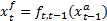
As the most used approach to handle the complexity of model mentioned above, the EKF-based method is to linearize (29), assuming a quasi-steady-state behavior of the system, it can be represented by Equation 31,
 (31)
(31)
where matrix  represents the transition speed between states; vector
  is related with the behavior tendency of the states. Dynamic State Estimation depends strongly on the forecasting technique chosen to estimate parameters, and
 . The technique used in this document for calculating and Linear exponential smoothing of Holt (online parameter identification technique) widely used to forecast the states in this type of work (Leite da Silva, Do Coutto Filho, and De Queiroz, 1983; Nguyen, Venayagamoorthy, Kling, and Ribeiro, 2013; Valverde and Terzija, 2011) which provides good predictions even when state variables are assumed to be independent. Values of these parameters can be obtained as in Equations 32 and 33,
 (32)
(32)
 (33)
(33)
where  is the predicted state vector at step
  ,
,  is the identity matrix, the parameters
 and
and  are between 0 and 1 in this work have been fixed constant throughout the whole simulation to 0.5 and 0.8 respectively as proposed in Valverde and Terzija (2011), and the vectors a and b can be obtained from previous (a priori) knowledge (Equations 34 and 35),
 (34)
(34)
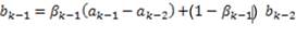 (35)
(35)
where is the predicted state vector and,  is the true state vector.
Active and reactive power balance, line flow equations and bus voltages govern the non-linear function h(∙) that relates measurement  with the state vectors. The flowchart for the EKF method is illustrated in Figure 3.
3. Results and discussion
The proposed calculation of the error ( ) and performance (
 ) indices, and their respective standard deviation are presented in Table 2 for 14 and 30 buses
Table 2 Index error for EKF and standard deviations ( ) for 14 and 30 buses
| Buses | Index | EKF | σEKF |
| 14 |

|
0.26995 0.40309 0.34899 0.72139 | 0.13941 0.17706 0.44329 0.07470 |
| 30 |
|
1.4533 1.9930 1.7524 0.84601 | 0.48266 0.75792 0.75503 0.06132 |
Table 2 shows that the average of the () index and the average errors of the 30-bus system are higher than the equivalent averages of the 14-bus system.
The Figures 4to8 show the evolution of error indices () and performance indices ( according to definitions established before for 14 and 30 bus systems
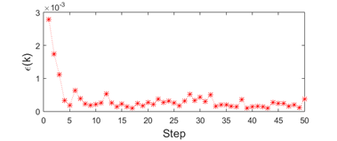
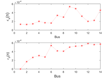


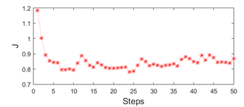
Figure 5 shows the voltage and angle magnitude error for each bus during the 50 steps of our simulation. Figure 4 and Figure 7 present the estimation error of each simulation step considering the 2n−1 state variables of each system. The performance index ( ), in Figure 6 has a peak in the first steps because of the difference between the initial estimated values and the true values of the measurements is high.
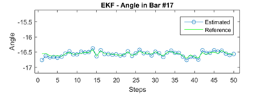
The Figures 9,Figure 10,Figure 11,Figure 12 show the behavior of the estimation values concerning the true values of voltage and angle magnitudes. It can be seen that in all the graphs there is a tracking of the estimation signal towards the real signal.


4. Conclusion and recommendations
In general, it can be concluded that the methodology used in this work to estimate states of an EPS is showing good results and the error indices reported can be accepted as referential values in this types of studies, e.g., to compare accuracies between different methods employed to state estimation of EPS. Future work will study the Monte Carlo methods deeply in the state estimation of EPS such as the Ensemble Kalman Filter and sequential Monte Carlo methods.

