Inglés (pdf)
 Articulo en XML
 Referencias del artículo
 Enviar articulo por email
 Citado por SciELO
  Similares en
SciELO
Similares en
SciELO 
 Permalink
1. INTRODUCTION
Speed profiles obtained by considering geometrical design of a road are very important input data for road safety analysis. A speed profile is a graphical representation of operational or design speeds along a road. Specifically, operative speed profiles use predictive speed models, according to individual geometrical features, e.g. horizontal curves.
In order to link all these speed models altogether, it is necessary to have speed change data or models that are capable of describing acceleration / deceleration process of a vehicle driving along many varying geometrical design elements, e.g. between tangents and curves, so as to interpret the driver’s behavior and his/her responding action upon vehicle speed when perceiving said features along the road.
Three main approaches for analyzing the above issue are found in the literature. The first approach considers a single and constant value for accelerations/decelerations; the second view regards different and constant values, whereas the third one takes into account acceleration / deceleration values that depend on road geometry.
The main difference among them is related to the way that speed transitions occur along the road: linear transitions associated to constant acceleration / deceleration, and non-linear transitions, for acceleration / deceleration dependent on road geometry. Without attempting to discern which approach is the most convenient one, it is possible to speculate that the description of the acceleration / deceleration process in terms of road geometry allows linking together the many instantaneous (point) operating speed estimations along the trajectory and, thus, enable for obtaining a continuous description of the driver’s speed selection.
Based on the above premises, this work is aimed at proposing acceleration / deceleration models for light-weight vehicles travelling along two-lane rural and mountain roads, using the experiences carried out on various roads of the Province of San Juan, Argentina. On a first stage, the field work on acceleration / deceleration estimation selected from the literature are briefly presented and discussed. This review leads to understanding in detail the aspects of acceleration measurement, data processing and modeling. A second stage describes the methodology used in data collection, selection of measurement sectors, drivers, measurement equipment and data processing. Upon finishing this step, the acceleration / deceleration performance patterns are analyzed, and finally, calibration and validation of the acceleration / deceleration models are discussed and conclusions are drawn.
2. BACKGROUND
Swiss Road Standards pioneered the use of acceleration / deceleration profile models to evaluate the consistency by observing the speed changes between consecutive horizontal curves design (VSS, 1991). Those standards assumed that acceleration / deceleration take place at the moment of approaching/exiting tangent and curves, as well as that vehicle speed remains constant within the circular curve. The acceleration / deceleration value is assumed constant at 0,8 m/s2. This approach was used by other researchers who built acceleration models that regarded constant values (Bester, 1981; Brodin & Carlsson, 1986; Lee et al., 1983; Watanatada et al., 1987; Figueroa y Tarko, 2005).
Lamm et al., (1988) chose 11 road stretches to study the deceleration pattern. This study considered deceleration from approach tangent into the curve and, conversely, the acceleration to exit the curve into the exit tangent. Results have indicated that the deceleration and acceleration starts/ends on a point located between 210 and 230 m from the start/end of the curve. They adopted an acceleration / deceleration rate equal to 0,85 m/s2. An Australian research team found accelerations in rural roads ranging from 0,34 to 1,18 m/s2 and deceleration from 0,50 to 1,47 m/s2 (McLean, 1991). Collins and Krammes (1996) studied 10 horizontal curves and approach/exit tangent on two-lane rural roads in Texas (USA). They aimed at evaluating the assumption that acceleration / deceleration when approaching/exiting a curve is constant and equal to 0,85 m/s2. The research concluded that this acceleration / deceleration rate is a reasonable value for curve-approaching deceleration, though it may overestimate the acceleration rates when exiting the curve.
In USA, studies made at 21 measuring sites resulted in acceleration rates ranging from 0 to 0,54 m/s2 and deceleration ones from 0 to -1,00 m/s2 (Fitzpatrick et al., 2000). The study establishes that operating speed of light vehicles are sensitive to longitudinal grades higher than ±4%, but the accelerations and decelerations could be sensitive to longitudinal grades higher than ±9%. On the other hand, in Chile, the ranges of acceleration were from 0,21 to 0,29 m/s2 and -0,15 to -0,65 m/s2 for deceleration on 32 horizontal curves in flat terrain (Echaveguren y Basualto, 2003). Hu and Donnell (2010) evaluated the results for night driving and they found acceleration / deceleration ranging from -1,34 to +1,31 m/s2.
Among the previous studies, road curvature is the most common variable that affects acceleration / deceleration, specially curve radius and driving speed and eventually the longitudinal grade (Bennett, 1994; Pérez et al., 2010). With regards to data collection equipment, most studies resort to point, on-the-spot, recording equipment, such as laser gun, radar gun, magnetic or piezoelectric sensors, etc. Only few studies employed continuous recording equipment, such as GPS-based recorders. The main disadvantage of point-recording equipment arises from the fact that stations are not placed where acceleration / deceleration maneuver starts or ends, because such points cannot be determined on a-priori basis. On the other hand, the continuous recording equipment could determine such spots with precision, though they may adversely affect the driver’s behavior by the feeling that the driver is being watched over. Video cameras have also been used and they have proved to be very useful equipment for data processing.
3. RESEARCH METHODOLOGY
3.1 Test Section
The selection of test roads considered the following criteria: (i) paved, two-lane rural roads; (ii) presenting no physical features that may affect the operative speed; (iii) presenting similar environmental conditions in all selected routes, (iv); presenting longitudinal slopes smaller than 8 %; (v) with good pavement conditions; and (vi) low traffic so as to ensure a free-flow driving. Based upon these criteria, three routes located in the Province of San Juan, Argentina were selected, namely RP-60 (San Juan – Ullum; 18,8 km), RN-40 (San Juan – Jáchal; 122,1 km), RN-149 (Talacasto – Pachaco; 89,0 km), which traverse areas classified as semi-mountainous, rolling, and mountainous, respectively, as described in the Table 1. In addition, these three roads covered a wide range of geometric variables, such as small to large curve radii, short to long tangents, and so on. These considerations help to generate more representative models.
Table 1. Characteristics of the test sections
| Characteristics | San Juan - Ullum | San Juan - Jáchal | Talacasto - Pachaco |
|---|---|---|---|
| Road code | RP60 | RN40 | RP149 |
| Road length (km) | 18,8 | 122,1 | 89,0 |
| # of curves | 34 | 63 | 246 |
| # of curves with posted speed | 1 | 5 | 11 |
| Posted speed values | 60 | 40 – 60 | 50 – 60 |
| Horizontal curve radii (R, m) | 123,5 – 883,1 | 287,0 – 3 429,4 | 26,5 – 6 349,1 |
| Deflection angles (Δ, º) | 2 – 92 | 1 – 76 | 0 – 164 |
| Horizontal curves length (L, m) | 26,1 – 468,4 | 20,2 – 744,6 | 13,1 – 936,5 |
| Grades (i, %) | -7 to +8 | -6 to +7 | -6 to +7 |
| Tangents (Lr, m) | 21,6 – 2 448,1 | 25,0 – 15 149,3 | 8,6 – 6 030,2 |
| Road lane width (m) | 7,30 | 7,30 | 7,30 |
| Terrain Type | Semi -mountainous | Rolling | Mountainous |
3.2 Driver team
Fourteen drivers, aged 21 to 53, and having from 3 to 40 years driving experience, participated in speed data collection. Twelve were men and two were women. They drove both ways along the selected road stretches, driving their own vehicles (cars and small pickups). The drivers were frequent travelers along these roads, to attend their business or work duties. All persons were told about the research’s aims and were specifically encouraged to drive as they normally do, following their own driving habits.
We assume that habitual drivers tends to drive at higher speeds and tolerate higher speed changes, in contrast to occasional drivers who drives at lower speeds and therefore it’s operating speed profile is more flat and the speed changes are lower. From the point of view of geometric design, the driving style of habitual drivers leads to this type of drivers are the fastest driver population and represents the worst condition.
To avoid biases due to the vehicle ability to accelerate and decelerate and considered mainly the effect of road geometry, when the driver were selected, was considered only drivers that owns light cars with ABS brake system in good conditions and with nominal engine power ranging between 100 and 170 hp.
3.3 Measuring Equipment
The recording equipment was a 10-Hz Video VBOX Lite featuring a built-in multi-camera system for obtaining geo-referenced digital images altogether with the collected data. The equipment captures on-move data referenced by an 8-satellite array which renders a very reasonable precision, with no need for a base station to perform corrections. Data is recorded every 0,1s, with travelled distances recorded with 0,05% precision, vehicle speed, with 0,2 km/h precision, ground altitude, with ± 10m precision, and heading, with 0,5° precision. The equipment can export data each 1, 5, 10 m, or another step length. Heading is related to driving trajectory changes, regardless vehicle speed. The Video VBOX Lite (data logger) equipment features a multi-camera recording system that allows overlapping real-time high-resolution images, thus easing the following step of data interpretation and analysis. It also counts with a Kalman filter algorithm that renders an efficient recursive solution based on the least-square method, allowing for data synchronization and data matching whenever a satellite blackout occurs.
3.4 Field data collection
The Video VBOX Lite kit is installed in the vehicle without any visual disturbance to the driver. The high-resolution camera is installed on the front windshield, headed to the road lane centerline, and it is plug in to the data logger. A second camera is installed above the right side (rider’s) seat so as to avoid any visual interference and to prevent as much as possible a feeling of being watched over while they are driving. The data logger is linked to a GPS antenna fixed to the vehicle’s roof. An accompanying person on the right-side seat controls the measuring and recording equipment. The measurements were made on daylight periods while drivers were driving in dry paved roads with fair weather.12
The most relevant data collected by Video VBOX Lite were: speed, horizontal position, relative altitude, heading and geo-referenced video recordings. The speed recording allows computing the longitudinal acceleration / deceleration. Horizontal positioning and heading allow estimating the road’s planimetry, whereas the relative altitude allows calculating the road’s longitudinal slope. Finally the geo-referenced videos allow estimating the sight distance over the road.
It was noticed, that during the tests, no driver felt disturbed by the test setting itself, because they were aware of the research objectives for habitudinal driving. This attitude was asserted by the fact that most drivers broke the speed limits, with some of them speeding up to 160 km/h.
3.5 Data processing
In advance to calculating the longitudinal acceleration / deceleration using the speed recordings by Video VBOX Lite, the equipment files’ data were processed to obtain a proper and useful database. Each file is subject to Kalman filtering so as to build a new database having less noise than the original source data.
Speed readings taken at 5 m distance were exported into the database. It was opted for this length because on such short distance, the vehicle speed does not change substantially. This way, the computational load is conveniently reduced. A 500 m distance on both run ends were deleted to account for personal driving habitat at his/her regular driving speed.
Some further 500 m lengths were deleted for pre- and post-intersection segments. All segments of tangents and /or curves where the vehicle had to do overtaking maneuverings were deleted because the driver’s overtaking behavior was not included in the study objectives.
All data where vehicle were not in free flow were discarded, considering a critical headway time of 6 s. This consideration allows ensuring that the studied speed readings were not affected by traffic. With this new database, the longitudinal acceleration / decelerations were computed.
To this aim, the approach/exit tangents to curves were broken down into 20 m segments, measured from the horizontal curve approach (PC-LT) and horizontal curve exit (PT+LT) points, up to the corresponding starting or ending point of each longitudinal segment at either side, i.e., approach/exit, of the curve. Because the GPS device capture data each 0,1 s, at the driving speed the 20 m length permitted to obtains enough data points per segment to estimate a probability distribution function, also to obtains different percentiles of speed, acceleration and /or deceleration in each cross section of the segmentation of Figure 1. The curves were dividing into four parts. The various partitions for tangents and the curve itself are shown in Figure 1. In order to compute the acceleration / deceleration value for each section of Figure 1, the following kinematics equation was used:
Where:
ai,i-1: acceleration / deceleration between consecutive points i and i-1, in m/s2,
Vi-1: speed at point i-1, in km/h,
Vi: speed at point i, in km/h, and,
di,i-1: distance between points i and i-1, in m.
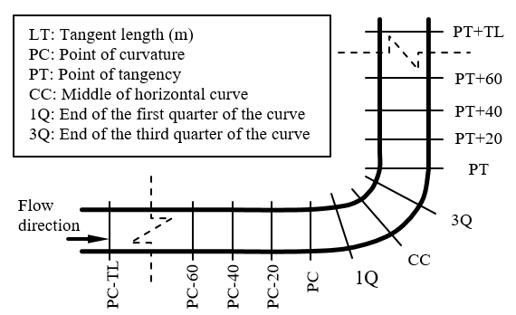
In Figure 1, PC represents the point at which the curvature starts to decrease and PT the point at which the curvature starts to increases. The distance between PC and PT represent the curve length, including the circular arc and the spirals (if exists) at both sides.
Two approaches were considered for acceleration / deceleration computing. The first one involves calculating the acceleration / deceleration from each individual run, and then computes the 85th percentile of acceleration. This percentile value was chosen by considering an analogy with the operative speed profiles. The second approach is compute the acceleration / deceleration values from the 85th percentile of speed.
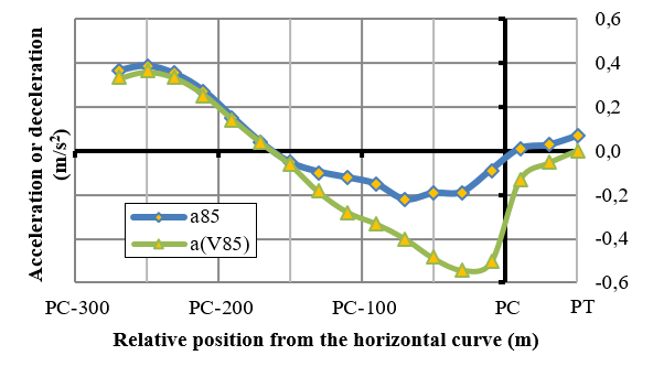
In order to define which one of these two methods is the most adequate one, several road stretches were analyzed through both approaches. For example, Figure 2 shows the calculation results made with Equation 1 for both approaches in the curve No. 17 on the San Juan-Jáchal road. It can be noted that there are differences between the 85th percentile acceleration profile, computed through individual runs (a85), and the acceleration profile obtained from the 85th percentile of the speed profile (a(V85)). Besides, marked discrepancies are also noted on the slope of the a(V85) profile, which could be associated to the fact that speed spread varies greatly on two consecutive sectors, especially when approaching or exiting a horizontal curve. By regarding these considerations, it was opted for the first approach, because it renders more precise acceleration / deceleration values than those of the second method.
4. SPEED CHANGE PATTERNS ANALYSIS
4.1 Deceleration before the curve
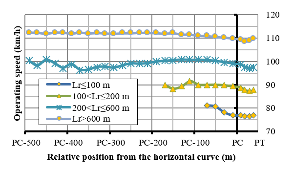
In order to find the deceleration starting point, an analysis was made on speed change at the approaching tangents before entering the horizontal curve. The operative speed was calculated for the various 20m-sections, computed from the beginning of the horizontal curve (PC) for all tangents of all studied roads. The average (mean) value of operative speeds was computed for tangent lengths, as classified into the following groups: <100 m; between 100 and 200 m; between 200 and 600 m; and for tangents longer that 600 m, as represented in Figure 3.
The acceleration / deceleration profiles for these four groups are plotted in Figure 4. These profiles indicate the average deceleration for each section; which are smaller than the typical ones appearing in the literature.
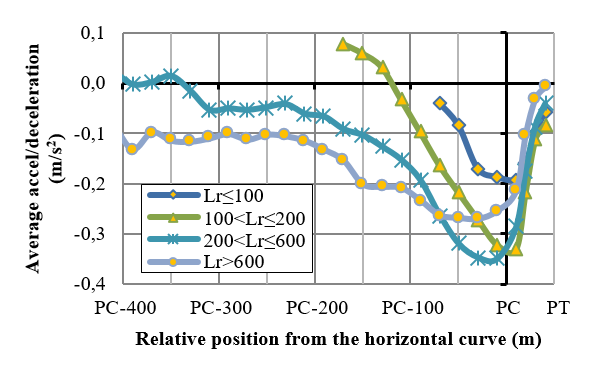
Figure 4. Average acceleration / deceleration for 4 groups of approaching segment of the horizontal curve
Figure 4 shows that the deceleration maneuver begins at the point where negative values arise. A t-test was conducted for each segment section, in order to verify whether the values differed from zero or not. This test permitted to determine the point where deceleration starts. According to this approach, a vehicle moving along a 200-600 m in tangents should start the deceleration maneuver at a distance of 230 m (measured from starting point of the curve, regardless its speed. From observations, nevertheless, it can be stated that the deceleration starting point for a vehicle moving with a speed lower than 80km/h is shorter than the proposed 230 m value. Considering that the tangent lengths affect the speed variations, it was decided to estimate the deceleration starting point as a function of speed. To this aim, the database of Figure 3 was used, and the results are included in the first rows in Table 2.
4.2 Ending deceleration and starting acceleration point
Deceleration starts at the beginning of the tangent and it ends somewhere inside to the curve. In order to find the location of such point, the horizontal curves were split into several radius ranges and each section were split in four sectors: curve’s starting segment (PC), ¼ curve length (1Q), curve center (CC), ¾ curve length (3Q) and curve end (PT). Each sector showed an operative speed average that is statistically different from those of adjacent sectors, as seen in Figure 5. For these sectors, the average acceleration / deceleration values were obtained, as shown in Figure 6.
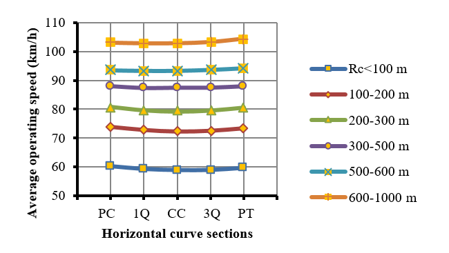
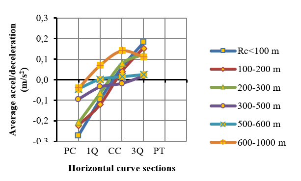
A t-test was carried out to determine which deceleration value was not different from zero, with 95% level of significance. It was found that deceleration ends at: the curve’s center on both horizontal curves having <300 m radius; at about ⅜ of the horizontal curve length for curve radii between 300-600 m, and for curves with radii >600 m, the deceleration ends at about ¼ of the horizontal curve length. In other words, when the curve radius is greater, the deceleration distance is shorter at the curve, as measured from the curve’s starting point. For higher radius (between 600 and 1000 m) the speed change pattern results different. In higher radius the acceleration and deceleration maneuvers are not so clear like in smaller radius. Possible due the fact that in higher radius, drivers can reach the desired speed and demands more visibility, which makes that they not need to accelerate when exit the curve and reduced slightly the speed.
4.3 Acceleration ending point
A similar analysis was made for identifying the acceleration’s end point. The exit tangent (Lrs) after the curve was sectioned into several sections for speed evaluation, considering for each section a different mean operative speed from those of contiguous sections (p<0,05), as shown in Figure 7. The average acceleration value was computed for each section of the tangent, as shown in Figure 8. Figure 8 shows that the most representative acceleration value is found around PT and that the acceleration maneuver ends at different places, depending on the exit segment. A t-test was performed in order to determine the location where the acceleration mean value was not statistically different from zero.
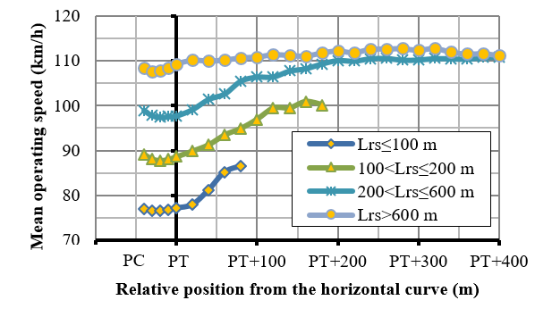
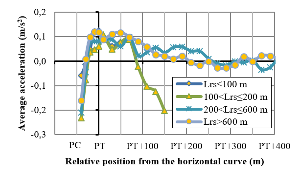
Figure 8. Average acceleration for various sectors of the exit segment after the ending point (PC) of the horizontal curve
Results show that the acceleration length, on the exit segment, is shorter than the deceleration starting point on the approaching segment to the curve. This could be linked to the fact that the driver, upon exiting a curve, wants to recover as fast as possible the speed lost in the previous maneuver, whereas on the deceleration maneuver, the driver starts slowing down along a longer distance, for better adjustment of vehicle speed before heading into the curve.
Is possible that in short tangents, the drivers when perceives a shorter length ahead, tries to gain speed at the beginning of the of the tangent but they do not have enough distance to continue accelerating because is approaching the next curve, so they need to decelerate. On the other hand, when a larger tangent exist between curves, driver do not need to decelerate immediately, until to estimate the minimum time and distance that considers enough to accommodate its speed before to entering to the next curve. This behavior occurs in horizontal reverse curves and depends of the value of the radii of each curve and of the tangent length between curves.
5. MODEL CALIBRATION
The study proceeded to analyze the influence of the following factors upon the representative deceleration: the longitudinal slope of homogeneous stretches; curve length; curve deflection; the drivers and curve radius and its transformations R0,5, 1/R and 1/R0,5.
5.1 Deceleration models
Since it is difficult to analyze an entire deceleration maneuver, it was decided to use a single representative deceleration value in evaluating the effect of road geometry upon the deceleration pattern. This representative value lies near the curve’s beginning, because it is there where the deceleration profile reaches its maximum value. In order to obtain this representative value, the deceleration’s 85th-percentile was computed for the distance between the starting deceleration point and that of the curve’s beginning, by applying equation (1).
The study proceeded to analyze the influence of the following variables upon the representative deceleration: the longitudinal slope of homogeneous stretches; curve length; curve deflection; the drivers and curve radius. On a first step the horizontal curve radius (R) was used, altogether with its transformations R0,5, 1/R and 1/R0,5. Results from regression analysis revealed that the 85th percentile for deceleration is significantly correlated with all R transformations. However, the variable which showed the best results was 1/R. The maximum deceleration obtained in this study was -1,45 m/s2. This value lies among the corresponding ones shown in the literature that ranges between -1,16 m/s2 and -2,5 m/s2 (Dell’Acqua and Russo, 2010; IHSDM, 2012). The deceleration models are shown in Table 2.
5.2 Acceleration models
From the speed pattern results, it was found that the most influential variables on the representative acceleration were the radius, length of the horizontal curve, and the longitudinal slope grade. This acceleration occurs at a point before exiting the horizontal curve, and it is the maximum value found for this acceleration maneuver. A correlation analysis helped in determining whether the length and/or the radius of the horizontal curve are correlated to the representative acceleration. Three radius transformations (R0,5, 1/R, 1/R0,5) and the curve length (L) were used. The results showed that the acceleration is significantly correlated (with a significance level of 95%) with all the above variables. Nevertheless, 1/R and L obtained the highest determination coefficient (R2=0,98) and the lowest RMS (RMS=0,18m/s2), respectively. Therefore, the model based on the curve length was discarded. The maximum acceleration obtained was 1,20 m/s2, which lies within the corresponding range reported in the literature that ranged between 0,54 m/s2 and 1,77 m/s2. Table 2 summarizes the acceleration models obtained.
5.3 Proposed models
The proposed acceleration / deceleration - geometry models, the acceleration / deceleration length modes and their validity ranges, are shown in xref Table 2.
Table 2. Summary of acceleration / deceleration-geometry and acceleration / deceleration length models proposed
| Alignment condition | Calibrated Model | N | R2 | RMS (m/s2) | Validity Range |
|---|---|---|---|---|---|
| Deceleration length on the approach tangent to the curve (Lid) | Lid = 70 | 38 | - | - | Lre≤100 m or V85≤85 km/h |
| Lid = 110 | 77 | - | - | 100<Lre≤200 m or 85<V85≤95 km/h | |
| Lid = 230 | 72 | - | - | 200<Lre≤600 m or 95<V85≤105 km/h | |
| Lid = 250 | 48 | - | - | Lre>600 m or V85>105 km/h | |
| Deceleration before the curve | 47 | 0,56 | 0,07 | 287<R<990 m and CCR≤50 º/km | |
| 103 | 0,56 | 0,14 | 39<R<883 m and CCR>50 º/km | ||
| End of deceleration/start of acceleration in the curve | Lfd = Lia=0,5L | 248 | - | - | R≤300 m |
| Lfd = Lia=0,375L | 203 | - | - | 300<R≤600 m | |
| Lfd = Lia=0,25L | 134 | - | - | R>600 m | |
| Acceleration before exiting the curve | 11 | 0,98 | 0,02 | 25<R<1000 m | |
| Acceleration length after exiting the curve | Lfa = 30 | 147 | - | - | Lrs≤100 m |
| Lfa = 30 | 67 | - | - | 100<Lrs≤200 m | |
| Lfa = 90 | 64 | - | - | 200<Lrs≤600 m | |
| Lfa = 130 | 43 | - | - | Lrs>600 m | |
| CCR: curve change rate (º/km).R: horizontal curve radius, mN: number of test sectionsLid: Length measured from the deceleration starting point on the approaching segment to the horizontal curve approach (PC) of the horizontal curve, m.Lre: Length from the approaching segment to the horizontal curve, m.d85 = 85th percentile of deceleration before entering the curve, m/s2.Lfd: Ending deceleration length on the horizontal curve, from the curve PC, m. Lia: Starting deceleration length on the horizontal curve, from the curve PC, m.a85 = average acceleration before exiting the horizontal curve, m/s2.Lfa: Length of acceleration end on the exit segment, from the horizontal curve exit (PT), m.Lrs: Length of the tangent segment at the curve exit, m. RMS: root mean square error, in m/s2.R2: determination coefficient | |||||
With regard to acceleration and deceleration rates in the Table 2, Fitzpatrick et al. (2000) also used the radius of the curve transformed (1/R2) as a predictor of deceleration in a range of radii between 175 and 873 m (-0,0008726 + 37430 / R2). For the rest of the decelerations, they used fixed values of 0,05 m/s2 and 1,25 m/s2 for radii greater than 873 m and less than 175 m, respectively. In addition, for acceleration, no predictor was used, it was only divided into radius ranges: R> 436 m (0.21 m/s2), 250 m ≤ R ≤ 436 m (0.43 m/s2), and R < 250 m (0.54 m/s2). On the other hand, other previous researches did not consider any variable to predict acceleration and deceleration rates, they used fixed values. Consider this facts, the present study is helping to expand understanding in this field.
It is important to clarify that although the results of Table 2 have been obtained from the collection of only three roads, they have together a length of 230 km, which covered a wide range of geometric variables. However, the results are only applicable within the ranges shown, on roads with longitudinal slopes less than 8% and with similar landscape conditions (desert). In addition, care should be taken with the results with low N values, especially with the acceleration model before exiting the curve.
6. CONCLUSIONS
Deceleration when approaching a horizontal curve is not constant, and depends on the inverse of the curve radius. Two equations were proposed to estimate the representative deceleration, namely, for CCR≤50º/km and CCR>50º/km, because they obtain better estimations than with just a single general equation.
The acceleration begins on the approaching segment to the curve and ends at an internal point of the horizontal curve. Therefore, if curve radius is high then deceleration tends to decrease within the curve.
The deceleration length before entering the curve depends on the tangent length previous to the curve and the approach speed into the curve.
The acceleration is not constant, and it starts before exiting the horizontal curve. The acceleration is dependent on the square root inverse of the curve radius.
The acceleration distance at curve exit is shorter than the deceleration distance on the approaching tangent. When exiting the curve, the driver wants to recover the lost speed as soon as possible.
The acceleration distance at curve exit is variable. As the curve exit tangent increases, the length of the acceleration tangent increases as well.
Results from regression analysis revealed that the 85th percentile for deceleration is significantly correlated with all R transformations. However, the variable which showed the best results were 1/R. Statistically significant relationships with other variables was not found, although the longitudinal slope should also influence the deceleration.
The results of this research, considering that they are more detailed than the previous ones, will help to calculate more precise operating speed profiles. These speed profiles can be used in consistency analysis, fuel consumption, capacity and service level analysis, cost of road users, among others.