


 Inglés (pdf)
 Articulo en XML
 Referencias del artículo
 Enviar articulo por email
 Citado por SciELO
  Similares en
SciELO
Similares en
SciELO 
 Permalink
1.INTRODUCTION
General Relativity is the theory used to describe gravitational phenomena, it provides impeccable agreement with observations. The Universe is modelled as a (3+1)-dimensional manifold (3 spacial dimensions and 1 time dimension). In this theory, the quanta associated with gravitational waves, i.e. gravitons, are massless particles with two independent polarization states, of helicity ±2 (Bergshoeff et al. (2009)). In order to have massive particles within the gravitational theory, alternative theories are needed and one should break one of the underlying assumptions behind the theory (de Rham (2014)).
On the other hand, if we consider a (2+1)-dimensional manifold, i.e., (2+1)-General Relativity, it has been proven there are no gravitational waves in the classical theory (Carlip (2004)). Also, it has no Newtonian limit and no propagating degrees of freedom (Carlip (1995)). But, in 1992, Bañados, Teitelboim, and Zanelli (BTZ), to great surprise, showed that in (2+1)-dimensional gravity there is a black hole solution (Bañados et al. (1992)).
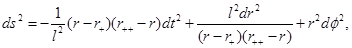
This solution is called the BTZ black hole, it has an event horizon and (in the rotating case) an inner horizon. This black hole is asymptotically anti-de Sitter, and has no curvature singularity at the origin, so it is different from the known solutions in (3+1)-dimensions as the Schwarzschild and Kerr black holes, which are asymptotically flat (Carlip (1995)).
The rotating BTZ metric is presented in Bañados et al. (1992) and it is given by Equation (1)
 (1)
(1)
where  and
and  with |J| ≤ Ml, where M and J are the mass and angular momentum that are defined by the asymptotic symmetries at spatial infinity. The parameter l is related with the cosmological constant as Λ = −1/l2. This metric is stationary and axially symmetric, with Killing vectors ∂t and ∂φ, and generically has no other symmetries (Carlip (2005)).
The event horizons of the BTZ black hole are located at  and there would be a naked singularity if |J| > Ml.
Also, if M = −1 and J = 0, it is the anti-de Sitter (AdS) space-time (Bañados et al. (1992)).
In this context, an alternative theory to General Relativity is New Massive Gravity (NMG), which is a theory that describes gravity in a vacuum (2+1)-spacetime with a massive graviton (Bergshoeff et al. (2009)). Some black hole solutions have been found for this theory, in particular rotating solutions, which are interesting in the search of geometric inequalities as the ones found for the Kerr black hole in (3+1)-General Relativity.
In Dain (2014) the known behaviour of the Kerr family is presented. Since the Kerr metric depends on two parameters, the mass m and the angular momentum J, it was shown that it represents a black hole if and only if the following remarkably inequality holds  . Otherwise the spacetime contains a naked singularity. So, there is an extreme Kerr black hole that reachs the equality
  and it represents an object of optimal shape (Dain (2014)). A graphical representation of the structure of a spatial slide of the Kerr black hole in the non-extreme case, which has two asymptotically flat ends, can be seen in Figure 1. For the extreme case, the corresponding representation is Figure 2, where it can be seen the asymptotically flat end, and also the cylindrical end, a typical feature of extreme initial data.
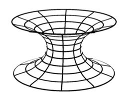
Figure 2 The cylindrical end on extreme Kerr black hole initial data. Picture taken from (Dain (2012)).
In this paper, we study a rotating black hole in NMG, considering specially its extreme limit with respect to the angular momentum parameter, as we are interested in its properties in the context of geometrical inequalities. The article is structured as follows. In section 2, we introduce briefly the NMG field equations. In section 3 some static black hole solutions are presented while in section 4 we present the rotating black hole solution that we analyse in this paper. In section 5 we perform our analysis of the non-extreme and extreme cases, in particular their event horizons, area of some surfaces and the distance to their horizons. Finally, in section 6 we discuss the conclusions of our analysis.
2.NEW MASSIVE GRAVITY
As we said before, in General Relativity, if we consider a (2+1) spacetime we will find that there are no propagating degrees of freedom for a massless graviton (de Rham (2014)). If we want to include a massive graviton that propagates degrees of freedom in the theory, we need an alternative theory. NMG is one of the alternatives (Bergshoeff et al. (2009)).
The action for NMG is 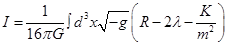 , where
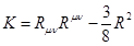 , and G is the equivalent gravitational constant in a (2+1)-spacetime, while m and λ are parameters related with the cosmological constant (Bergshoeff et al. (2009); Oliva et al. (2009)). If the scalar K is equal to zero, then the action of General Relativity is obtained, or if m2 → ∞.
So, as shown in Oliva et al. (2009), the vacuum field equations in this alternative theory are of fourth order and read
 (2)
(2)
where Kµν is a tensor defined as Equation (3)
 (3)
(3)
and K = gµνKµν . Black hole solutions have been found for the field equations in Equation (2), we present some of them in the next section.
3.STATIC BLACK HOLE FAMILIES
From Bergshoeff et al. (2009), NMG theory generically admits solutions of constant curvature given by  with two different values of the parameter Λ, determined by
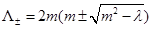 . This means that at the special case defined by m
2 = λ the theory possesses a unique maximally symmetric solution of constant curvature given by
. This means that at the special case defined by m
2 = λ the theory possesses a unique maximally symmetric solution of constant curvature given by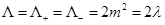 . In that case, the theory admits the following Euclidean metric as an exact solution (Oliva et al. (2009))
 (4)
(4)
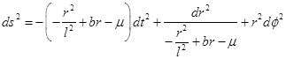
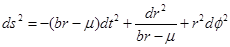
where b and µ are integration constants, and Λ = 2λ is the cosmological constant. This solution is asymptotically of constant curvature Λ. The parameter b is not related with the mass or the angular momentum of the black hole, so it is considered a hair parameter.
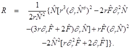
From the metric in Equation (4), the curvature scalar R is  . This means that, unlike the BTZ solution, the metric has a curvature singularity at the origin. Depending on the value of the cosmological constant, we have the following kinds of solutions:
Solutions with Λ< 0
If we call  and make the following coordinates transformation ψ → it, φ → ϕ in Equation (4), we obtain the solution
 (5)
(5)
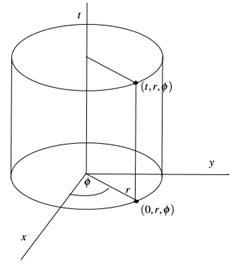
for the NMG field equations, where −∞< t < +∞, 0 < ϕ < 2π and r > 0. In Figure 3 the coordinates used in metric in Equation (5) are shown. It can be seen there are two spacial coordinates, r and ϕ, and one temporal coordinate, t. This coordinate system is used throughout the present article. This solution describes an asymptotically AdS black hole with an inner and an outer event horizon, r − and r +, such that the metric in Equation (5) can be written as presented in Equation (6)
 (6)
(6)
and the parameters are given by  and
and . In the case of b = 0, the solution reduces to the static BTZ black hole. It was found the parameter b determines the causal structure of the black hole (Oliva et al. (2009)).
Solutions with Λ> 0
If we now call  , i.e., a positive cosmological constant, and then we make the same type of coordinate transformation ψ → it, φ → ϕ in Equation (4), we obtain the solution
 (7)
(7)
which describes an asymptotically de Sitter (dS) black hole. It has two horizons, r ++ and r +, where r + is the event horizon which is surrounded by the cosmological horizon r ++ (Oliva et al. (2009)). The metric in Equation (7) can be written as the one presented in Equation (3.2)
and the parameters are given by 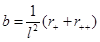 and
and  . In this case, the parameter µ needs to satisfy the following inequality
Solutions with Λ = 0
NMG admits solutions without cosmological constant and constant curvature. In that case, the metric is given by Equation (8)
 (8)
(8)
with an event horizon at  .
.
4.ROTATING BLACK HOLE
A rotating extension of the asymptotically AdS black hole was presented in Oliva et al. (2009). For that case, the solution is the metric
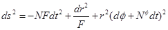 (9)
(9)
with the functions defined in Equations (10), (11), (12), (13) and (14) as follows
 (10)
(10)
 (11)
(11)
 (12)
(12)
 (13)
(13)
 (14)
(14)
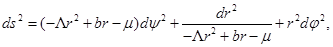
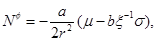
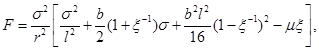
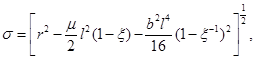
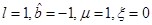
where the angular momentum is given by J = Ma, M is the mass (measured with respect to the zero mass black hole) and the parameter µ is related with the mass as µ = 4GM. In this metric, the angular momentum parameter a satisfies −l < a < l. The extreme case for this solution would be when the condition |a| = l is satisfied, but it is not possible to attain this limit with the metric in the form in Equation (9), given that ξ = 0 in this case and the terms ξ −1 in the metric diverge.
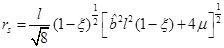
Because of our interest in studying the extreme case of a rotating black hole in NMG theory, a change in the parameter b is needed. As proposed in Giribet et al. (2009), the parameter  is defined as
  , and the metric in Equation (9) takes the form
 (15)
(15)
with the functions defined in Equations (16), (17), (18), (19) and (20) as follows
 (16)
(16)
 (17)
(17)
 (18)
(18)
 (19)
(19)
 (20)
(20)
The metric in Equation (15) is the one presented in Giribet et al. (2009), where the rotational parameter satisfies −l ≤ a ≤ l and the extreme case |a| = l is included.
It can be noticed that making the change 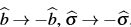 , takes the functions to themselves, that is
 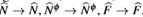 . Therefore, this change does not present new metrics, and we take only σ ≥ 0 (non-negative branch), which is also the right choice for the BTZ case (b = 0).
ANALYSIS OF THE NON-EXTREME ANDEXTREME ROTATING BLACK HOLE
In this section we analyse some features of the rotating black hole presented in Equation (15), as the singularity, the event horizon, the area of some surfaces in the manifold and finally, the distance to the horizon for radial curves, with emphasis in the geometry of the extreme case. Quantities that refer to the extreme case will be denoted with a subscript e.
Curvature singularity
We calculate the curvature scalar,
 (21)
(21)
Therefore, from Equation (21), we have a curvature singularity if , and this happens when
 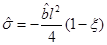 , which means, as
  , that
 , and the singularity is located at
 (22)
(22)
and, from Equation (22), we have as constraint , where
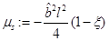 . As
. As  is the BTZ black hole, then there is no curvature singularity.
Event Horizon
As can be seen in Equation (15), the event horizon is located where , that is, where
 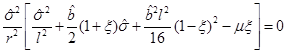 is satisfied. This is achieved if
 (23)
(23)
or
 (24)
(24)
If Equation (23) is satisfied, then we have that the following  could be the location of the event horizon. On the other hand, the condition in Equation (24) is equivalent to
 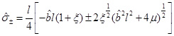 and so, the event horizon is at
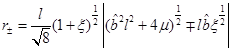 .
.
It means there are three possible roots of  , but we are interested in the outer horizon and its relation to the curvature singularity, so it is necessary to determine which of the roots is larger. In order to
  we have to require
  .This condition is less restrictive than the condition to ensure
  . Now it is necessary to separate the analysis according to the sign of
  .
.
If, then 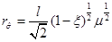 and
and 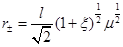 , with the constraint
 . We have that
  . As
. As  then
then  . Also, we have that
  which tells us that in general
  ,
,  and that
  only if µ = 0 or ξ = 0.
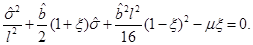
So we conclude that the mass needs to satisfy the condition µ ≥ 0, that the outer horizon is  , and that has a simple root in r+ unless µ = 0 or ξ = 0, in which case it has a double root. We see that r+ is an increasing function of µ and also an increasing function of ξ.
Being more explicit regarding the multiplicity of the roots, if ξ > 0 and µ > 0 then  and
and  , which shows that has a simple root at r+.
r2
If µ = 0 then the solution does not depend on ξ and , which is the massless BTZ black hole.
 If ξ = 0 and µ> 0 then
  and
and , which shows that
  has a double root at r+.
These results are summarized in Figure 4. Each point in the figure represents a metric with a value of µ and a value of ξ. The allowed values of these parameters are µ ≥ 0 and 0 ≤ξ ≤ 1, and the nature of the biggest root of for each combination of parameters has been made clear by the color coding.
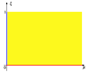
Figure 4 Parameter space for : (a)The blue line represents the massless BTZ black hole, the horizon is a double root of . (b)The region shaded in yellow represents non-extreme BTZ black holes, the horizon is a simple root of. (c)The red line represents extreme rotating BTZ black holes, the horizon is a double root of

If then  and . Therefore we need to compare r+ with rσ. To have
  we need
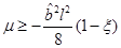 , which is more restrictive than
  , and we have
 . Also, we see that
  and that
  only if
  or
or  .
.
So we conclude that the mass needs to satisfy the condition , that the outer horizon is
 , and that
  has a simple root in r+ unless µ = µ0 or ξ = 0, in which case it has a double root. In general r+ > 0, and r+ = 0 only if µ = µ0 and ξ = 0. We see that r+ is an increasing function of µ and also an increasing function of ξ.
Being more explicit regarding the multiplicity of the roots, if ξ > 0 and µ>µ0 then  and , which shows that has a simple root at r
+.
and , which shows that has a simple root at r
+.
If ξ > 0 and µ = µ
0 then and r
+
> 0, which shows that has a double root at r
+.
and r
+
> 0, which shows that has a double root at r
+.
If ξ = 0 and µ>µ
0 then and r
+
> 0, which shows that has a double root at r
+.
If ξ = 0 and µ = µ
0 then and in this case r
+ = 0, which seems to imply that F diverges, but in fact has a double root at r
+, as can be seen by taking a Taylor expansion of σ
b near r = 0. These results are summarized in Figure 5.
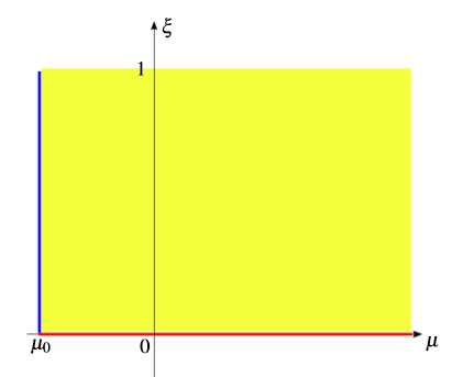
Figure 5 Parameter space for : (a)The blue line represents black holes with minimum mass µ0, the horizon is a double root of . (b)The region shaded in yellow represents non-extreme black holes, the horizon is a simple root of . (c)The red line represents extreme rotating black holes, the horizon is a double root of and coincides with the curvature singularity.
With regard to the singularity, if µ ≥ µs then r + ≥ rs . In order for r + = rs we need ξ = 0, that is, to be in the extremely rotating case. So in general the singularity is hidden behind the horizon, unless we are in the extremely rotating case, and then the singularity and the event horizon coincide.
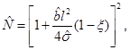
In the extreme case, |a|=l, we have
ξe
= 0 which can be replaced in the formula above or we can obtain the horizon from  , where
 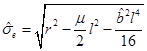 . The condition
  is satisfied if
 (25)
(25)
or
 (26)
(26)
If Equation (25) is satisfied, we have  while if Equation (26) is true, then re+ = re− and re+ can be written as
 (27)
(27)
Given that  must be satisfied, the mass satisfies µ ≥ µ
0. This condition is also presented in Giribet et al. (2009).
must be satisfied, the mass satisfies µ ≥ µ
0. This condition is also presented in Giribet et al. (2009).
On the other hand, it also can be proven by algebraic calculations that  and so, the outer horizon is given by Equation (27) in the rotating extreme case. Additionally, one can prove that
  and the equality is obtained only in the extreme case.

If then . In order for
  we need that
 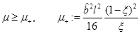 . Then
  and
and  only if µ = µ+. On the other hand, if
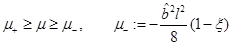 , then
  , and it is the outer horizon. Then
  can be written as
  , but the analysis of the multiplicity of the roots is not as straightforward as before.
So we conclude that we have two regions for the mass, if 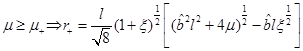 , and if
  .
.
It can be proved that if µ+ ≥ µ ≥ µ−, r+ is a decreasing function of ξ, in constrast with the case bb < 0. If µ ≥ µ+, the behaviour of the function r+ is a bit more complicated: if µ>µm, then r+ is an increasing function of ξ while if µ<µm, then r+ is a decreasing
function of ξ, where 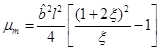 .
.
We concentrate now on the multiplicity of the outermost root of. If  and
and  then
then  and
and , then has a simple root in
  .
.
If and  then
then  and
and , , and therefore we have
  and
and  where
where  . This shows that has a root that behaves as
  when
when .
.
If  then
then  and
and , and therefore
  and
and , where
 (28)
(28)
So  has a simple root at
 .
.
If µ = µ
− then and  , and therefore
  and
and  , and
, and  has no root. These results are summarized in Figure 6.
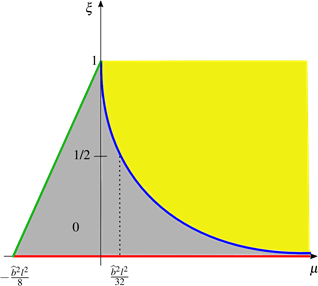
Figure 6 Parameter space for: (a)The blue line represents black holes with mass µ
+, the horizon is a root of . (b)The region shaded in yellow represents non-extreme black holes, the horizon is a simple root of . (c)The region shaded in grey represents non-extreme black holes, the horizon is a simple root of . (d)The red line represents extreme rotating black holes, the horizon is a simple root of . (e)The green line represents black holes with minimum mass µ−, has no zero.
Area of the black hole
If we consider the hyper-surface t = t 0, where t 0 is a constant, we have that the induced metric in the hyper-surface is
 (29)
(29)
Then, we consider the hyper-surface of t =t 0 at r = r 0, where r 0 is a constant. We have that the induced metric in the hyper-surfaces is
 (30)
(30)
In this hyper-surface, we are interested in calculating the area. From Equation (30), the area differential is  and, given that
 , the total area is
 , which corresponds to the length of a circumference of radius
 . At the extreme case, the area of the rotating black hole is
 .
.
As r 0 ≥ r +, if we denote by A + the area of the black hole, we have that A ≥ A +, and it is equal if and only if r 0 = r +.
If we consider the case b b ≤ 0 and fix the mass µ, as we have re + ≤ r +, then A + ≥ Ae +, where Ae + is the area of the extreme black hole, and it is equal if and only if r + = re +, that is in the extreme case. It means the horizon area in the extreme case is the area minimizer for the family of black holes.
For the case, given the different behaviours of r
+ depending on the values of µ, the area minimizer is different for each case. If , then the minimum area corresponds to the black hole with the smallest angular momentum. On the other range of values, where
 , the minimum area is obtained as follows: if
 , then it is obtained in the static case; if
 , then the area as a function of
  has two critical points, where
  corresponds to the local minimum for the area; and finally, if
 , then the minimum area is in the case where
 . As we have seen, the behaviour of the area in the
  case is more complicated that the one for the
  case and the extreme case is never the minimizer of the area of the black hole.
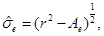
Distance to the horizon
For calculating the radial distance to the horizon, it is necessary to take the hyper-surface
 Then, the radial distance from a point at
  to a point at
  is
is  .
.
In particular, we want to calculate the distance from the event horizon to an arbitrary point r1 in the non-extreme and extreme
case, that is,  and
and
A quick argument allows us to see that for , L
+ is finite while
Le
diverges.
, L
+ is finite while
Le
diverges.
As r
+ is a simple root of we have that
 (31)
(31)
which is bounded and Equation (31) proves that L
+ is finite. On the other hand,
re
+ is a double root of , and then
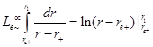 (32)
(32)
which is unbounded and Equation (32) proves that Le diverges. This shows that the extreme limit has a cylindrical end.
The same argument can be applied to the b > 0 case, showing that the distance to the horizon is always bounded, therefore not having an extreme limit in the sense of having a cylindrical end.
Although lengthy, L
+ and
Le
can be obtained in closed form, and we do it for b
b ≤ 0, as it corresponds to the case in which we are most interested. We start noticing that, from the metric in Equation (15), can be written as
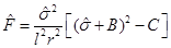 (33)
(33)
where  ,
, 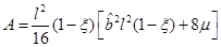 ,
,  and
and
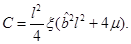 (34)
(34)
We can notice, from Equation (34), that C ≥ 0, it is C > 0 in the non-extreme case and C = 0 in the extreme case. Therefore, the distance between a point at r 1 and a point at the outer horizon r + in the non-extreme case is shown in Equation (35)
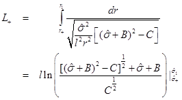 (35)
(35)
Where  and
and . From Equation (33), this can be written as Equation (36)
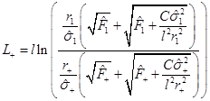 (36)
(36)
where  and
and . Given that
 , then L
+ is given by Equation (37)
, then L
+ is given by Equation (37)
 (37)
(37)
This shows that for the non-extreme case L + is bounded. We can also see that in the extreme limit, i.e., C → 0, L + diverges.
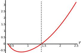
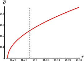
In Figure 7 can be seen the plot of as a function of r for the non-extreme case with , while in Figure 8 can be seen the plot of for the same values of the parameters. It can be noted that
  after the outer horizon, represented by the dashed line, and that is positive and bounded away from zero for r > r+.
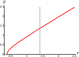

In Figure 9 we present the plot of the distance to the horizon as a function of r for the non-extreme case, again with 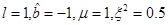 .
.
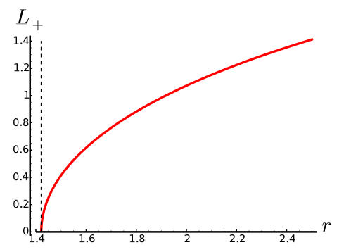
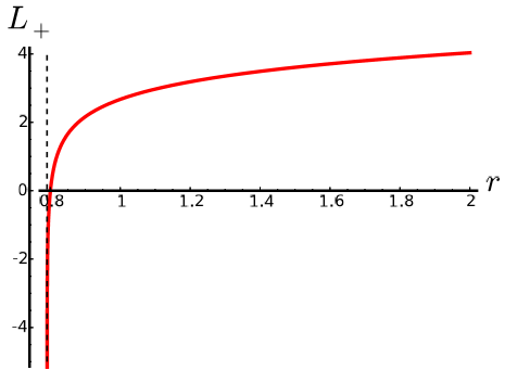
Also, in Figure 10 the metric structure near the horizon has been ploted. That is, the plot faithfully represents distances near the horizon. Here the similarity with the structure of the non-extreme Kerr black hole in (3+1)-General Relativity, represented in Figure 1, is evident.
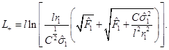
On the other hand, for the extreme case we have
 (38)
(38)
where
 Therefore, the distance between a point at r
1 and a point at the outer horizon
re
+ is given by Equation (39)
Therefore, the distance between a point at r
1 and a point at the outer horizon
re
+ is given by Equation (39)
 (39)
(39)
where  and
and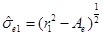 . From Equation (38), this can be written as
 (40)
(40)
where  and
and . Given that
 , then
Le
is unbounded. That is, the outer event horizon in the extreme rotating black hole is located at infinite distance from any point in the hypersurface.
, then
Le
is unbounded. That is, the outer event horizon in the extreme rotating black hole is located at infinite distance from any point in the hypersurface.
In Figure 11 can be seen the plot of  as a function of r for the extreme case with
 , while in Figure 12 can be seen the plot of
  for the same values of the parameters. It can be noticed that as in the non-extreme case,
  after the outer horizon, represented by the dashed line, and that is positive and bounded away from zero for
  .
.


In Figure 13 we present the plot of the radial distance to the arbitrarily chosen point r = 0.8 as a function of r for the extreme case with the same values of the parameters as before, namely, 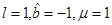 , and we see how the distance diverges at the horizon. Also, in Figure 14 the metric structure near the horizon has been ploted. As in the non-extreme case, this is a faithfull representation of distances near the horizon, and it can be seen directly the similarity with the structure of the extreme Kerr black hole in (3+1)-General Relativity, represented in Figure 2.

5.CONCLUSIONS
The different cases of a rotating black hole in NMG were analysed. This family of black holes has several interesting features and resembles closely black holes in (3+1)-General Relativity. In particular, the black hole can have several horizons, or none and then it describes a naked singularity.
The singularity and the horizon were analysed, showing different features depending on the sign of the hair parameter .
.
Of particular interest to us is the case ≤ 0, in the sense that it has an extreme limit with respect to the angular momentum parameter. We calculated the distance to the horizon in the non-extreme and extreme cases, showing that in the non-extreme case it is finite while in the extreme case it diverges. This shows that the initial data for the black hole changes structure from black hole initial data to trumpet initial data. This same change occurs in the Kerr spacetime in (3+1)-General Relativity.
Also, the area of the horizon was calculated, showing that, being the other parameters fixed and  ≤ 0, the minimimum of the area occurs for the extreme case. This again coincides with what happens in the Kerr spacetime.
These characteristics make this black hole a suitable candidate for conjecturing geometrical inequalities in NMG, playing the role that Kerr had for geometrical inequalities in (3+1)-dimensions.


