Inglés (pdf)
 Articulo en XML
 Referencias del artículo
 Enviar articulo por email
 Citado por SciELO
  Similares en
SciELO
Similares en
SciELO 
 Permalink
Introduction
Water is the most abundant natural resource on the planet; its quantity is approximately 1.385 billion km3. Out of this overall volume, as little as 1% is usable freshwater; 81% of it is present in glaciers and polar zones, while the remaining 18% is distributed among soil moisture, lakes, atmospheric vapor, rivers, and living organisms (Bitsch et al., 2021). All lifeforms on our planet, including flora, fauna, and human beings, have developed due to water availability (Singh, Yadav, Pal, & Mishra, 2020). Ecuador possesses a significant quantity of water resources; its average total runoff is 43,500 m3 per inhabitant a year, four times greater than the world average of 10800 m3 per inhabitant (Machado, dos Santos, Alves, & Quindeler, 2019). Water quality is at risk due to human activities near water sources. These activities are usually related to urban areas, mining areas, oil exploitation, and agriculture. These activities generate pollutant discharges with high concentrations of organic matter, nitrogen, phosphorus, heavy metals, and hydrocarbons (Ustaoğlu, Tepe, & Taş, 2020). Agricultural activity is extensive in the province of Chimborazo due to favorable climatic and geographical conditions (Moreano-Logroño & Mancheno-Herrera, 2020). In the last ten years, the Guano River has been used mainly in agricultural activities; in its course, it receives sanitary, agricultural, and industrial discharges. In addition, its flow has been reduced by 50%, changing the water quality and affecting the balance of the aquatic ecosystem, the soil, and people’s health (Shakir, Chaudhry, & Qazi, 2012).
To study the characteristics of water resources, quality indexes are used to verify whether the water complies with the specifications for its intended use; in addition, the effects of pollutants need to be assessed (Akhtar et al., 2021; Gupta & Gupta, 2021; Nong, Shao, Zhong, & Liang, 2020; Uddin, Nash, & Olbert, 2021; Villa-Achupallas, Rosado, Aguilar, & Galindo-Riaño, 2018). These indexes allow researchers to gather information on trends and identify river disturbances sources. Additionally, these indexes are necessary to study the characteristics of water resources and their quality to ensure the balance between human activities and the water ecosystem (Rivera, Encina, Muñoz-Pedreros, & Mejias, 2004). The US National Sanitation Foundation - water quality index (WQI-NSF) is used worldwide for this type of study. This method referred to here as Ramirez’s approach, is based on characteristics of North American rivers, which relate physical-chemical variables to average weights assigned to each for evaluating the specific pollution type (Gradilla-Hernández et al., 2020; Nugraha, Cahyo, & Hardyanti, 2020).
Works carried out in the area it is shown that the Guano River is affected by human activities, such as the excessive use of water for irrigation and the reception of wastewater (Castillejos & Arévalo, 2018; Castillo-López, Salas-Cisneros, Logroño-Veloz, & Vinueza-Veloz, 2021; Cevallos, 2015; Quevedo, 2020). But in these works, contamination is not related to other characteristics present in the area, such as geomorphology and flow.
Therefore, this work proposes a novel study to determine the water quality of the Guano River, using a variation of the WQI-Dinius that includes variables such as the average slope and the river’s flow. In addition, this work compares the results obtained with this variant in the index with WQI-NSF and WQI-Dinius.
Methodology
Sampling sites
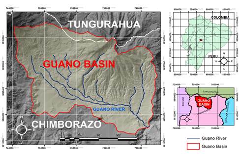
The Guano River basin (Figure 1) is located in the Ecuadorian highland between Tungurahua and Chimborazo; the river is the product of the thaws from Chimborazo’s volcano and the runoffs generated in the Igualata moorland. The river’s source is downstream of Andaluza, in the area of Llío, where the Agags and Puluchaca streams merge at 3090 masl. The Guano River flows from northwest to southeast and runs into the Chambo River after traveling 21 km. Runoff from slopes in the area feeds the Guano River on its course (Chidichimo et al., 2018).
According to the vegetation cover and the use of the soil (Table 1), the main anthropic activity is agriculture since it has a higher percentage of the area than the rest of the micro basin areas. In addition, the rate of population area corresponds mainly to the town of Guano, which sits on the banks of the river and is the one that shows the most significant interference in its quality. To determine the sampling points, vegetation and land use information (Mendoza et al., 2021) were analyzed (Table 1). The river was traversed from the upper part to the river mouth, corroborating what was identified in the characteristics of land use and vegetation data.
Table 1: Area of the vegetal coverage and use of soil.
| Vegetal coverage and use of soil | Area (km 2 ) |
|---|---|
| Natural forest | 3.60 |
| Crops | 277.58 |
| Grass | 28.01 |
| Paramo | 69.44 |
| Cities | 5.65 |
In addition, the anthropic activities that affect the environmental conditions of the same are identified from the preliminary information on the cover and soil use. The river was explored from the mouth, identifying the characteristics of vegetation cover and soil use and the human activities that affect the river’s environmental conditions; thus, 29 observation points of anthropic activities were found (Table 2).
Table 2: Observation points of anthropic activities with their UTM coordinates.
| Code | Description | X | Y | Masl. |
|---|---|---|---|---|
| P_RIVER 1 | Guano river, Llío | 754395 | 9826549 | 3120 |
| P_CHANNEL 1 | Irrigation Channel 1 | 759572 | 9822858 | 2800 |
| P_DISCHARGE 1 | Wastewater discharge Colegio Pérez Guerrero | 761098 | 9822398 | 2760 |
| P_DISCHARGE 2 | Wastewater discharge 80 m before the town of Guano1 | 761646 | 9822235 | 2725 |
| P_DISCHARGE 3 | Waste water discharge beginning of the town of Guano | 761717 | 9822241 | 2720 |
| P_DISCHARGE 4 | Waste water discharge 70 m downstream | 761753 | 9822178 | 2720 |
| P_DISCHARGE 5 | Waste water discharge 25 m downstream | 761774 | 9822169 | 2720 |
| P_DISCHARGE 6 | Waste water discharge 27 m downstream | 761799 | 9822159 | 2720 |
| P_DISCHARGE 7 | Waste water discharge 25 m downstream | 761857 | 9822135 | 2720 |
| P_DISCHARGE 8 | Discharge of wastewater before the town of Guano | 761891 | 9822121 | 2720 |
| P_SLOPE 1 | Spring Park of the slopes | 761940 | 9822074 | 2720 |
| P_SLOPE 2 | Spring Park of the slopes | 761969 | 9822046 | 2720 |
| P_DISCHARGE 6 | Discharge of residual water 40 m after the park of the slopes | 762003 | 9822014 | 2720 |
| P_SLOPE 3 | Spring Park of the slopes | 762029 | 9822004 | 2720 |
| P_DISCHARGE 7 | Discharge of residual water 40 m after the park of the slopes | 762057 | 9821994 | 2720 |
| P_SLOPE 4 | Spring Park of the slopes | 762093 | 9821980 | 2720 |
| P_DISCHARGE 8 | Discharge of residual water 40 m after the park of the slopes | 762122 | 9821969 | 2720 |
| P_SLOPE 5 | Spring Park of the slopes | 762179 | 9821922 | 2720 |
| P_RIVER 2 | Guano River, before Pebble Spinning Mill | 762877 | 9821879 | 2680 |
| P_DISCHARGE 9 | Wastewater discharge Pebble Spinning Mill | 763684 | 9821858 | 2680 |
| P_RIVER 3 | Guano River, before unloading Santa Teresita sector | 763959 | 9821894 | 2673 |
| P_DISCHARGE 10 | Waste water discharge Santa Teresita | 764249 | 9821860 | 2640 |
| P_RIVER 4 | Guano River, before the Chingazo Canal - Pungal | 765041 | 9821806 | 2640 |
| P_CHANNEL 3 | Canal Chingazo - Pungal | 765533 | 9821776 | 2607 |
| P_SLOPE 6 | Spring of the Elenes | 765959 | 9821465 | 2600 |
| P_SLOPE 7 | Spring of the Elenes | 766022 | 9821436 | 2600 |
| P_DISCHARGE 13 | Wastewater discharge San José Alto | 767236 | 9819720 | 2560 |
| P_DISCHARGE 14 | Waste water discharge Quimiac sector | 767383 | 9819519 | 2556 |
| P_RIVER 5 | Guano River, before the mouth of the Chambo River | 769511 | 9817696 | 2480 |
From these sampling points: P_RIVER1, P_RIVER 2, P_RIVER 3, P_RIVER 4, and P_RIVER 5 were selected to determine the water quality of the Guano River concerning the interference of human activities. In addition to these sampling points, by areas, from the upper part to the mouth of the river. Once these sampling points were chosen, over the time frame encompassing July to November 2018 (dry season), the water samples were taken in triplicate for 18 days at each monitoring point, giving 240 pieces for water quality analysis. All models were collected by the authors manually in plastic containers. For the physical-chemical parameters, the bottle (1000 mL) was submerged 20 cm below the water surface with the peak of the bottle in the direction of the current until filled the bottle free of bubbles that may form at the mouth of the bottle. For the microbiological analysis, 100 mL of sample was taken in a sterile plastic container (Rice, Baird, & Eaton, 2017).
Parameters used in the indexes
Laboratory analysis for water was performed according to the Standard Methods for the Examination of Water and Wastewater (23rd ed.) (Rice et al., 2017) as described below:
The Electrometric Method 4550-H+ B for pH was carried out with a Model HI99121 pH meter, using a model HI1230B electrode by HANNA INSTRUMENTS of Woonsocket, Rhode Island, United States, which enables a measuring range from pH 2.00 to 16.00. The method consists of shaking a 100 mL aliquot of water to ensure homogeneity. Then the electrode is immersed in the sample for 1 min and the pH value is read when the equipment stabilizes.
The Electrical Conductivity Method 2510 B was performed using a Model SEVEN COMPACT CONDUCTIVITY S230 conductivity meter, with an electrode Cond probe InLab 710 by METTLER TOLEDO of Greifensee, Switzerland. The range of measurement was from 0.001 to 1000 mS/cm. The method involves shaking an aliquot of 100 mL of water to ensure homogeneity. Then, the electrode was immersed in the sample for 1 min, and the conductivity value was read when the equipment stabilized.
The Total Dissolved Solids Method 2540 C was conducted with the previous equipment, with a measuring range from 0.00 mg/L...1000 g/L. The method involves shaking an aliquot of 100 mL of water to ensure homogeneity. Then the electrode is immersed in the sample for 1 min, and the total dissolved solids value is read when the equipment stabilizes.
The Membrane Electrode Method 4500-O G for determining Dissolved Oxygen was carried out with the Model HI98198 OD and a model HI764113 electrode by HANNA INSTRUMENTS of Woonsocket, Rhode Island, United States; the measuring range was from 0.00 to 50 mg/L. This method consists of introducing the electrode into the river bed so that the water covers the electrode membrane completely. The equipment is allowed to stabilize for 1 min, and the optical density (OD) value is reported as a concentration in mg/L.
The Nephelometric Method 2130 B for determining Turbidity is carried out with a Model HI93703 (HANNA INSTRUMENTS of Woonsocket, Rhode Island, United States) with a measuring range from 0.00 a 1000 FTU. This method involves gently agitating the sample for 1 min; then the sample is poured into the cell of HANNA INSTRUMENTS HI93700d tr of Woonsocket, Rhode Island, United States. The turbidity value is read when the equipment stabilizes and all air bubbles disappear.
A modified phosphates Method 4500-P-E was applied with a range of 0.02 to 2.50 mg/L PO4 -3. This method is carried out with the spectrophotometer HACH DR 5000 of Loveland, Colorado, United States, using sample cells of 10 mL (HACH 2495402 5000 of Loveland, Colorado, United States). This method involves gently agitating the sample for 1 min before placing it into the cell. Then, the contents of one PhosVer3 Reagent Powder Pillow (HACH, catalog number: 2106069 5000 of Loveland, Colorado, United States) is added to the cell; a blue color develops if phosphorus is present in the sample. If so, the sample cell should be closed immediately and shaken vigorously for 20-30 s. After this, the sample should be allowed to stand still for 2 min. Next, start program 490 P with the spectrophotometer set to a wavelength of 880 nm. Insert the blank into the cell holder, push zero, and the display shows 0.00 mg/L PO4 -3. Then, the prepared sample cell is cleaned with reagent, and the prepared sample is inserted into the cell holder; results are displayed in mg/L PO4 -3.
The Nitrogen Method (Nitrate) 4500 NO3 - E modified to HACH method 8039 had a measuring range from 0.3 to 30.0 mg/L NO3 -. This method is carried out with a HACH DR 5000 spectrophotometer and Model HACH 2495402 sample cells of 10 mL 5000 of Loveland, Colorado, United States. This method involves gently agitating the sample for 1 min. Then, the sample is placed in the cell, and the contents of one NitraVer 5 Reagent Powder Pillow are added. The sample cell was closed immediately, shaken vigorously for 60 s, and let to still stand for 5 min. Next, prepare the blank and fill it in a second sample cell. Start program 355 N with wavelength set to 500 nm. Zero the instrument for the blank, clean the sample cell with reagent, and introduce the sample into the cell holder; results will be shown in mg/L NO3 -.
EDTA Titrimetric Method 2340 C for Total hardness (mgCaCO3/L). This method needs 25 mL of sample. First, one adds to the sample 1 to 2 mL buffer solution (ammonium chloride and ammonium hydroxide) to give a pH of 10.0 to 10.1. Next, 1 to 2 drops of indicator solution or an appropriate amount of dry-powder indicator formulation (Eriochrome Black T -NET) are added. Add standard EDTA (0.01M) titrant slowly, under continuous magnetic stirring, until the last reddish tinge disappears. The last few drops should be added at 3 to 5 s intervals. At the endpoint, the solution typically turns blue.
The Titration Method 2320 CB for Alkalinity (mgCaCO3/L). In this method, 25 mL of sample 1 to 2 drops indicator solution (Methyl Orange) are added and titrated with a standard 0.1 N sulfuric acid solution. The reagent should be added slowly, under continuous stirring, until the sample color changes to purple.
Biochemical Oxygen Demand (BOD) 5210 B. 5-Day BOD modified to VELP BOD EVO Sensor of Usmate, Italy; for this measurement, one used a BOD sensor set consisting of a BOD Sensor, a dark glass bottle, an alkali holder to absorb the carbon dioxide, and a stirring bar. BOD (mg/L) value will be obtained directly from the display at any time, even after five days. For 5 days, the set is kept in an incubator VELP SCIENTIFICA FOC 120I at 20 °C in Usmate, Italy. Then, a magnetic stirrer is inserted in an amber glass bottle (500 mL), and the BOD sensor is installed. The sensor reports that the value after 5 days is the one that determines the BOD5.
Chemical Oxygen Demand (COD) 5220 D, Closed Reflux, Colorimetric Method. One used HACH DR 5000 spectrophotometer 5000 of Loveland, Colorado, United States. Samples were gently agitated for 1 min and held in a vial reagent HACH LR (range 3-150 mg COD/L) at an angle of 45º. A clean pipet was utilized for dispensing 2.00 mL of sample to the vial. The same procedure was used for another vial filled with deionized water and utilized as the blank. After closing the vial it should be held by the cap, over a sink. The content of the vial can be mixed by inverting the vial gently several times. Next, vials are placed in A preheated DRB200 reactor for 2 h at 120 ºC. After turning off the heat, vials should cool in the reactor for 20 min to 120 ºC or less and then cool to room temperature in a tube rack. The spectrophotometer should be set at 420 nm, and 430 COD LR program should be started. Samples are recorded relative to the blank, and results are displayed in mg/L COD.
Membrane filter technique for members of the coliform group 9222 modified to Petrifilm Coliform Count Plate of Northern Minnesota, United States. This method consists of gently agitating samples for 1 min and placing Petrifilm Coliform Count Plates on the surface. Lift the top film and, with Pipettor or equivalent held perpendicularly to the plate, place 1 mL of sample or diluted sample onto the center of the bottom film. Prevent pushing sample off film to avoid entrapping air bubbles. Do not let top film drop. With the flat side down, place 3MTM PetrifilmTM Spreader on top film over inoculum. Gently apply pressure on the 3M Petrifilm Spreader to distribute inoculum over a circular area before the gel is formed. Do not twist or slide the spreader. Lift 3M Petrifilm Spreader. Wait a minimum of 1 min for the gel to solidify. Incubate plates clear side up in stacks of up to 20. It may be necessary to humidify the incubator MEMMERT model BE500. 3M Petrifilm Coliform Count Plates can be counted using the 3MTM Petrifilm Plate Reader on a standard colony counter or other illuminated magnifiers. Colonies may be isolated for further identification. Lift the top film and pick the colony from the gel.
The flow was obtained with the float method, this is based on the speed-area principle, where (n) cross-sectional areas (depth and width) were measured, and the velocity was obtained from the time the float takes to travel a distance (5m). The Manning coefficient corrects the flow (Davids et al., 2019). Flow information of the different sampling points was obtained according to equation (1).
Where: Q is the flow rate (m3/s), V is the velocity (m/s), AT is the transverse area (m2), K is a correction factor (Manning coefficient) for rivers with a depth greater than 15 cm.
From the heights of the contour lines, the tool-created TIN is used to develop the digital terrain elevation model (DEM). Owing to the transform tool of TIN, the elevation raster of the study area is generated. From this raster, the Spatial Analysis slope tool is used to spatially determine the Slope (Sc) in the basin. This is done in the ArcGis 10.1 software (Mendoza et al., 2021).
Water Quality Indexes
In this study, the river course was divided into transects according to the natural conditions and the human activities present, leaving five monitoring points for studying the water quality; these points were chosen based on the pressure on different transects, as shown in table 2. The methodology of the water quality indices applied at the sampling points is described below.
The first methodology is the WQI-NSF, proposed by the National Sanitation Foundation; this is used to assess changes in water quality in specific sections of rivers at different times. The calculations of this method were carried out by weighting according to the parameter type (Table 3); that is, a percentage value was assigned to each parameter analyzed, their total sum being 1. This value was then transformed into a percentage value, with a range from 0 to 100 (Akhtar et al., 2021; Gupta & Gupta, 2021; Mukate, Wagh, Panaskar, Jacobs, & Sawant, 2019; Uddin et al., 2021; Ustaoğlu et al., 2020). Finally, equation (2) was used to calculate the WQI.
where W i is the weighting coefficient for parameter i, I is the index for each parameter, and n is the total number of parameters.
Table 3 Parameter of quality index WQI-NSF (Akhtar et al., 2021; Gupta & Gupta, 2021; Mukate et al., 2019; Uddin et al., 2021; Ustaoğlu et al., 2020)
| Parameter | Weigth |
| DO | 0.17 |
| Faecal Coliforms | 0.16 |
| pH | 0.11 |
| BOD | 0.11 |
| Nitrates | 0.10 |
| Phosphates | 0.10 |
| Temperature | 0.10 |
| Turbitity | 0.08 |
| Dissolved solids | 0.07 |
The second methodology described by Dinius determines the water quality of the sample according to the degree of water pollution. Thus, it will have a quality index close to 0 for utterly contaminated water. The index will be 100 for water with excellent conditions (Hoseinzadeh, Khorsandi, Wei, & Alipour, 2015; Mukate et al., 2019; Zotou, Tsihrintzis, & Gikas, 2019, 2020). Subsequently, this index indicates that a correction should be made to the results (Table 4). Each parameter has a weighting value of W that allows obtaining the corresponding WQI; the weight for each parameter was given in table 4.
Table 4 Parameter of WQI-Dinius (Hoseinzadeh et al., 2015; Mukate et al., 2019; Zotou et al., 2019, 2020)
| Parameter | I for WQI calculation | W for WQI calculation |
| Dissolved Oxygen - OD | 0.82*OD + 10.56 | 0.109 |
| Chemical Oxygen Demand - COD | 108 (COD)-0.3494 | 0.097 |
| Total Coliforms - CT | 136 (ColiTotal)-0.1311 | 0.090 |
| Fecal Coliforms -CF | 106 (EColi)-0.1286 | 0.116 |
| Conductivity | 506 (SPC)-0.3315 | 0.079 |
| Chloride | 391 (CL)-0.3480 | 0.074 |
| Total Hardness | 552(Hardness)-0.4488 | 0.065 |
| Alkalinity | 110(Alc)-0.1342 | 0.063 |
| pH < 6.9 | 100.6803+0.1856(pH) | 0.077 |
| pH = 6.9 - 7.1 | 1 | |
| pH > 7.1 | 103.65+0.2216(pH) | |
| Nitrates | 125(N)-0.2718 | 0.09 |
| Color Pt-Co | 127(Color)-0.2394 | 0.063 |
| Turbidity | 102.004-0.382|Ta-Ts| | 0.077 |
The numerical evaluation of the WQI-Dinius is obtained from the geometric mean (Equation (3)):
where W i are the specific weights assigned to each parameter (i), and weighed between 0 and 1, so the sum is equal to 1. Q i is the quality of the parameter (i), which depends on its concentration, and is rated from 0 to 100. PI represents the multiplication of the variables Q elevated to power W.
To contemplate the geomorphology and flow of the Guano River in the calculation of water quality, the WQI-Dinius was modified; therefore three steps were considered: (i) selecting the parameters, (ii) determining the sub-indexes, and (iii) determining the index by aggregation (Mukate et al., 2019; Samboni et al., 2007). For this purpose, the selection of parameters was separated into groups as follows: (a) organic matter: dissolved oxygen in % saturation and mg/L, biochemical oxygen demand and chemical oxygen demand, (b) bacteriological matter: total coliforms and fecal coliforms, (c) physical characteristics of water: color, Turbidity and electrical conductivity, (d) inorganic matter: alkalinity, hardness, chlorides, hydrogen ion concentration (pH), suspended solids, and total dissolved solids, (e) nutrients: nitrates, nitrites, phosphates, total phosphorus, and sulfates, (f) geomorphology characteristics: mean average of the Slope, Slope of the river course in the area under study, and flow. To apply the WQI-Dinius Modified, equation (4) was used. The I values were obtained from table 4, and the geomorphological characteristics (I) are equal to 1. The importance of W (WQI- Dinius Modified) for this method are described in table 5.
where Wi is the weighting coefficient for parameter i, I is the index for each parameter, and n is the total number of parameters.
The importance of parameter groups is identified for this case. Then the importance of the parameters within the parameter group is identified and the weight value is given at the end
Table 5: Weighing (W) for WQI- Dinius Modified.
| Importance between groups | Parameter | Weighing (W) Dinius | Importance between parameters | Weighing (W) WQI- Dinius Modified |
|---|---|---|---|---|
| 1 | Dissolved Oxygen | 0.109 | 1 | 10.9 |
| COD | 0.097 | 2 | 9.7 | |
| 2 | Fecal Coliforms | 0.116 | 1 | 11.6 |
| Total Coliforms | 0.09 | 2 | 9 | |
| 3 | Flow | - | 1 | 7.25 |
| Average slope of the main cause | - | 2 | 6.45 | |
| 4 | Nitrates | 0.09 | 1 | 9 |
| 5 | Conductivity | 0.079 | 1 | 7.9 |
| Turbidity | 0.077 | 2 | 7.7 | |
| pH | 0.077 | 1 | 7.7 | |
| Total Hardness | 0.065 | 2 | 6.5 | |
| Alkalinity | 0.063 | 3 | 6.3 |
The criteria that were used to determine the quality of the water once calculated with the WQI-NSF, Dinius-WQI, and modified WQI are shown in table 6 (Akhtar et al., 2021; Gradilla-Hernández et al., 2020; Gupta & Gupta, 2021; Hoseinzadeh et al., 2015; Mukate et al., 2019; Nong et al., 2020; Nugraha et al., 2020; Uddin et al., 2021; Ustaoğlu et al., 2020; Zotou et al., 2020, 2019). The results obtained by this methodology are analyzed according to the information in table 5 to identify whether the quality is excellent or bad as endpoints of the valuation.
Table 6: General criteria of WQI (Akhtar et al., 2021).
| Type of use | Color | Evaluation range | Quality description | Treatment |
| USE IN AGRICULTURE | E | 90-100 | EXCELLENT | It does not require purification to be consumed |
| A | 79-90 | ACCEPTABLE | Minor purification is needed for crops that require high water quality | |
| LC | 50-79 | SLIGHTLY CONTAMINATED | Treatment required for most crops | |
| C | 30-50 | CONTAMINATED | Treatment required for most crops | |
| FC | 20-30 | STRONGLY CONTAMINATED | Use only in very resistant crops | |
| EC | 0-20 | EXCESSIVE | Inacceptable for irrigation |
Results
The geomorphology of the Guano River (Table 7) shows that the micro-basin is small according to the area. The average slope of the micro-basin is medium-rough, the sections of the leading cause have medium-rough slopes in the upper part, and the lower part has gentle slopes.
Table 7: Geomophology of the Guano river.
| Parameter | Initials | Unit | Value |
|---|---|---|---|
| Area | A | km2 | 384.28 |
| Perimeter | P | km | 94.26 |
| Length of the main channel | Lc | km | 39.15 |
| The average slope of the basin | Sm | % | 13.74 |
| The average slope of the main channel | Sc | % | 16.35 |
| Slope first section | Sc1 | % | 11.2 |
| Slope the second section | Sc2 | % | 3.93 |
| Slope third section | Sc3 | % | 0.07 |
| Slope fourth section | Sc4 | % | 2.59 |
| Slope the fifth section | Sc5 | % | 2.39 |
In the high areas, the Guano River has an average flow of 0.68 m3/s, reaching the mouth with a flow of 1.83 m3/s. The flow decreases in the central region because there are irrigation channels along the river that redirect water from the river’s natural course (Table 8). Still, the flow recovers because springs provide additional fresh water to the river. Moreover, the physical-chemical and microbiological parameters that constitute the WQI were analyzed and performed for the five sampling points, as shown in Tables 9, table 10, table 11, table 12, and table13.
Table 8: Average flow of the Guano river at the sampling points (m3/s).
| Sampling | P_RIVER 1 | P_RIVER 2 | P_RIVER 3 | P_RIVER 4 | P_RIVER 5 |
|---|---|---|---|---|---|
| Sampling 1 | 0.79 | 0.97 | 0.94 | 1.83 | 2.14 |
| Sampling 2 | 0.81 | 0.99 | 0.96 | 1.87 | 2.19 |
| Sampling 3 | 0.60 | 0.74 | 0.71 | 1.39 | 1.63 |
| Sampling 4 | 0.73 | 0.90 | 0.87 | 1.70 | 1.99 |
| Sampling 5 | 0.75 | 0.92 | 0.90 | 1.74 | 2.04 |
| Sampling 6 | 0.56 | 0.69 | 0.66 | 1.29 | 1.51 |
| Sampling 7 | 0.68 | 0.84 | 0.81 | 1.58 | 1.85 |
| Sampling 8 | 0.70 | 0.86 | 0.83 | 1.62 | 1.90 |
| Sampling 9 | 0.52 | 0.64 | 0.62 | 1.20 | 1.41 |
| Sampling 10 | 0.64 | 0.78 | 0.76 | 1.47 | 1.72 |
| Sampling 11 | 0.65 | 0.80 | 0.77 | 1.51 | 1.76 |
| Sampling 12 | 0.48 | 0.59 | 0.57 | 1.12 | 1.31 |
| Sampling 13 | 0.59 | 0.73 | 0.70 | 1.37 | 1.60 |
| Sampling 14 | 0.61 | 0.74 | 0.72 | 1.40 | 1.64 |
| Sampling 15 | 0.73 | 0.90 | 0.87 | 1.70 | 1.99 |
| Sampling 16 | 0.83 | 1.02 | 0.99 | 1.93 | 2.26 |
| Sampling 17 | 0.85 | 1.05 | 1.02 | 1.98 | 2.31 |
| Sampling 18 | 0.63 | 0.78 | 0.75 | 1.47 | 1.72 |
Table 9: Results of the physical-chemical and microbiological analysis in P_RIVER 1.
Table 10: Results of the physical-chemical and microbiological analysis in P_RIVER 2.
Table 11: Results of the physical-chemical and microbiological analysis in P_RIVER 3.
Table 12: Results of the physical-chemical and microbiological analysis in P_RIVER 4.
Table 13 Results of the physical-chemical and microbiological analysis in P_RIVER 5.
| Sampling | pH | Conductivity | Temperature | Dissolved Oxygen | Turbidity | STD | Phosphate | Nitrate | Total hardness | Alkalinity | BOD | COD | Total Coliforms | Fecal Coliforms |
| - | µS/cm | ºC | mg/L | NTU | mg/L | mg/L | mg/L | mg CaCO3/L | mg CaCO3/L | mg O2/L | mg/L | ufc/100 mL | ufc/100 mL | |
| 1 | 7.16 | 590 | 18.96 | 6.15 | 7.07 | 333 | 1.05 | 16.42 | 276 | 51.41 | 1.79 | 15.87 | 189 | 52.00 |
| 2 | 7.20 | 573 | 17.28 | 5.73 | 7.67 | 339 | 1.91 | 10.76 | 294 | 46.23 | 2.03 | 25.88 | 141 | 24.00 |
| 3 | 7.02 | 590 | 18.63 | 4.84 | 11.09 | 333 | 1.04 | 11.25 | 275 | 46.23 | 1.56 | 15.53 | 197 | 33.00 |
| 4 | 7.08 | 623 | 21.08 | 4.60 | 12.69 | 334 | 0.95 | 10.90 | 255 | 47.27 | 1.47 | 11.39 | 391 | 56.00 |
| 5 | 6.36 | 629 | 19.84 | 5.51 | 16.60 | 367 | 1.18 | 25.67 | 287 | 53.13 | 3.46 | 20.01 | 236 | 56.00 |
| 6 | 7.03 | 894 | 20.80 | 5.51 | 10.94 | 445 | 2.08 | 22.05 | 371 | 50.95 | 1.76 | 19.67 | 346 | 59.00 |
| 7 | 6.96 | 761 | 19.87 | 4.04 | 9.83 | 529 | 0.86 | 8.11 | 287 | 44.23 | 2.67 | 20.01 | 241 | 54.00 |
| 8 | 6.46 | 924 | 20.87 | 4.75 | 12.40 | 819 | 1.09 | 11.80 | 375 | 45.37 | 2.89 | 18.98 | 295 | 61.00 |
| 9 | 7.03 | 616 | 17.90 | 7.07 | 9.49 | 377 | 1.17 | 21.68 | 303 | 56.44 | 1.93 | 17.54 | 250 | 69.00 |
| 10 | 7.07 | 599 | 16.23 | 6.66 | 10.09 | 384 | 2.14 | 14.21 | 323 | 50.76 | 2.19 | 28.59 | 186 | 31.00 |
| 11 | 6.89 | 616 | 17.57 | 5.76 | 13.51 | 377 | 1.16 | 14.85 | 302 | 50.76 | 1.68 | 17.16 | 260 | 44.00 |
| 12 | 6.95 | 649 | 20.02 | 5.52 | 15.11 | 379 | 1.06 | 14.39 | 280 | 51.90 | 1.58 | 12.58 | 516 | 74.00 |
| 13 | 6.23 | 654 | 18.78 | 6.43 | 19.02 | 412 | 1.32 | 33.88 | 315 | 58.34 | 3.73 | 22.11 | 311 | 74.00 |
| 14 | 6.90 | 919 | 19.75 | 6.43 | 13.36 | 490 | 2.33 | 23.15 | 407 | 55.95 | 1.50 | 21.73 | 457 | 78.00 |
| 15 | 6.83 | 787 | 18.82 | 4.96 | 12.25 | 574 | 0.96 | 10.70 | 315 | 48.56 | 2.89 | 22.11 | 318 | 72.00 |
| 16 | 6.33 | 950 | 19.82 | 5.68 | 14.82 | 864 | 1.22 | 15.57 | 412 | 49.81 | 2.56 | 20.97 | 389 | 81.00 |
| 17 | 6.90 | 642 | 16.85 | 7.99 | 11.91 | 422 | 1.32 | 28.61 | 332 | 61.97 | 2.11 | 19.38 | 330 | 91.00 |
| 18 | 6.94 | 625 | 17.28 | 7.58 | 12.51 | 429 | 2.40 | 18.76 | 355 | 55.74 | 2.05 | 31.59 | 245 | 41.00 |
Figure 2 shows the mean values obtained through the three indices for July to November 2018. The values are between 59 and 73. It is observed that July presents high values and October low values. Once the samples were analyzed, the quality index was determined via three methods, as described, for each sampling point (Table 14). The results show two types of quality and water, acceptable (A) and slightly contaminated (LC), predominating the LC classification in the three indices for type A.
Table 14: Results of WQI index for the Guano River.
| SAMPLE | WQI-NSF | WQI-Dinius | WQI-Dinius Modified |
|---|---|---|---|
| Sampling 1 | A | A | LC |
| Sampling 2 | LC | A | LC |
| Sampling 3 | LC | A | LC |
| Sampling 4 | LC | A | LC |
| Sampling 5 | LC | LC | LC |
| Sampling 6 | LC | A | LC |
| Sampling 7 | LC | LC | LC |
| Sampling 8 | LC | LC | LC |
| Sampling 9 | A | LC | LC |
| Sampling 10 | LC | A | LC |
| Sampling 11 | LC | A | LC |
| Sampling 12 | LC | LC | LC |
| Sampling 13 | LC | LC | LC |
| Sampling 14 | LC | LC | LC |
| Sampling 15 | LC | LC | LC |
| Sampling 16 | LC | LC | LC |
| Sampling 17 | LC | LC | LC |
| Sampling 18 | LC | LC | LC |
Discussion
According to the results, the Guano River is a small micro-basin, with slopes ranging from medium-rough to gentle. It also shows the results of the slopes in the sections studied since the river slopes range from medium-rough to soft. In addition, it is observed that the flow at the sampling points varies depending on human activities and natural conditions. In the upper part of the river (P_RIVER 1), the flow is small; at point P_RIVER 2, it increases a little due to the effect of the runoff of the sector. From point P_RIVER 3 the flow decreases, because there are irrigation canals (Castillo-López et al., 2021; Mendoza et al., 2021; Quevedo, 2020). P_RIVER 4 and P_RIVER 5 show an increase in the flow due to the presence of a spring that again provides water to the river (Chidichimo et al., 2018). Moreover, the water quality results also depend on anthropic and natural conditions. In other matters, the water quality results also depend on the anthropic and natural conditions.
From a geomorphological point of view, it is evident that the slope influences the water quality because the effect of the slope on the rivers is essential; it allows the self-purification of the water with high slopes (Marimón-Bolívar, Jiménez, Toussaint-Jiménez, & Domínguez, 2021; Šaulys, Survile, & Stankevičiene, 2019; Toussaint-Jimenez, Marimon-Bolivar, & Dominguez, 2020).
This is perceptible in the water quality in the upper part of the river, where there are medium-rough slopes, allowing the presence of surface runoff, oxygenation of the water, and the dissolution of pollutants. The slope is gentle in the middle and lower part of the river, minimizing self-purification conditions. In addition, 88% of the river area is affected by agricultural activity, extending from 3000 to 2480 masl. The actions of towns (San Andres and Guano) are notoriously detrimental to the water quality by wastewater discharges directly into the riverbed.
Furthermore, Guano's artisan activities, such as leather and textile garment making, produce organic contaminants, including detergents, dyes, and heavy metals. Furthermore, non-technical agriculture has deteriorated the water quality indicators. This includes the riparian forests, which have disappeared almost entirely from the river banks, causing erosion and drag of the materials (Quevedo, 2020). In this context, the water quality assessment was carried out at the five sampling points of the fundamental cause; the values shown are the average of the 5 points. The qualitative evaluation of the water quality of the Guano River is: WQI-NSF values acceptable (A) in 2 samples and slightly contaminated (LC) in the rest of the samples. WQI-Dinius values seven samples as good (A) and 11 as slightly soiled (LC). In the case of the modified WQI, the evaluation is somewhat contaminated (LC) in all the samples. That is to say; water treatment is necessary to improve its condition so that it should not affect the quality of the crops.
Conclusions
The three indices reveal that the water is slightly contaminated and must be treated before use. The WQI-Dinius Modified gives lower values concerning the other two indices, as it shows the effects of flow and slope in determining water quality. When there is less flow and the water is contaminated in areas of human activity, such as areas with wastewater discharge. In this context, the water Quality with WQI-NSF and WQI-Dinius has been used and validated in several rivers worldwide. Therefore, the results obtained with these indices for the Guano River are considered valid, showing that the river is slightly contaminated.
The study of the water quality of the Guano River allowed us to see the approximation to reality of the WQI-Dinius modified since when comparing them with WQI-NSF and WQI-Dinius, the results are lower. Still, the qualitative assessment is similar regarding the water quality along the river. In the same way, it was possible to assess how the slope and flow parameters affect the value of the WQI-Dinius Modified since it was noticed that there is a more significant contamination in the areas with slope and low flow, other areas with higher flow and greater slope. In the lower part of the river, the water quality improves due to the greater volume of water and the presence of springs, which allows the dilution of pollutants and oxygenation of the water.
Although the index shows somewhat different values, it should be studied in greater detail, with a more significant number of physical-chemical data, for several years and in other rivers with similar characteristics. In the same way, the sampling of the parameters should be carried out in the dry season, where there is less flow. The effect of the flow and the slope on the self-purification of the river water would probably be observed better: This is because the slope and the flow are new parameters in the WQI that need further study for the method to be reliable. In addition, the results in rivers already studied must be validated to verify if this can contribute to improving this type of water quality study.