Introduction
Lotfi Zadeh introduced fuzzy logic in the mid-sixties. Its use in various branches of science has been incessant, and of course, the applications in process control are numerous (Kavsek-Biasizzo, Skrjanc, & Matko, 1997). The term "Fuzzy" comes from the English word "fuzz," which denotes the lint covering the chicks' body when leaving the egg. This English term means "confusing, blurry, undefined, or out of focus." (Reznick, 1997).
The concept of fuzzy logic is widespread; it is associated with how people perceive the environment; for example, ideas related to a person's height, the speed with which an object is moving, the prevailing temperature in a room, are formulated ambiguously daily and depends on who perceives the physical effect or chemical, will be your statement about such a phenomenon. A person can be tall or short; something can move fast or slow; a temperature can be low or moderate or high. These statements about a variable are ambiguous because fast, low, high are statements by the observer. These may vary from one observer to another. For example, you can ask when something is hot or cold, how low the temperature is when We say cold, or how high it is when we say hot.
Fuzzy sets precisely define these ambiguities and are an extension of the classical set theory, where an element belongs or does not belong to a set, such element has only two possibilities, to belong or not, an item is bi-valued they are not defined ambiguities. With fuzzy sets, an attempt is made to model the ambiguity with which perceives a variable. Fuzzy sets are the basis for fuzzy logic, of the same So classical set theory is the basis for Boolean logic. With the fuzzy sets, logical if-then statements are made, defining these with Fuzzy Logic. This theme is typical of artificial intelligence, where it is tried to emulate in human thought. Our field of study is industrial control; we have to consider the operator's experience or knowledge base; this will be useful to emulate the human behavior with a machine, despite being very limited.
The incorporation of fuzzy logic into control systems gives rise to what we call fuzzy control systems. There are two major areas within the control systems: modeling or identification and control itself or direct control. First, we focus on process control, assuming the model of this is known. The idea is straightforward; it is about logically determining what should be done to achieve the control objectives best possible from a human operator's knowledge; without this basis, it is impossible to develop an application and make it work properly.
The references to applications of fuzzy logic that can be found in the literature are pervasive. Below is a very brief summary to put into perspective the broad scope of application of the theory of fuzzy logic.
In 1972 E. Mamdani used the theory of fuzzy logic and the expert knowledge of workers to design a diffuse controller that properly handled a laboratory steam engine (Kavsek-Biasizzo, et al., 1997). In 1976 H. Zimmermann employed fuzzy logic in decision-making problems, evaluating applications to bank loans (Reznick, 1997). Finally, in 1980 Holmblad implemented a diffuse controller for an industrial furnace. It constituted the first permanent industrial application of fuzzy Logic ( Menzl, Stuhler, & Benz, 1996). In 1982 M. Dohnal raised the possibility of modeling complex chemical engineering processes, using models based on fuzzy logic and linguistic variables (Chen, 1997). In Japan, in 1984, fuzzy logic was used to control chemicals in a water treatment plant. In addition, diffuse control systems were also implemented in Sendai city's underground network. In this case, the diffuse control system was responsible for taking the train up to the predetermined speed and keeping it in this condition, regardless of the geographical features of the route (curves, ascents, descents, etc.), and then stopping gently at the destination site (Henson & Seborg, 1994 ; Ha, Nguyen, Rye, & Durrant-Whyte, 1998). In 1985 M. Togai and H. Watanabe developed the first fuzzy logic chip. This work showed the implementation of an inference system based on the maximum-minimum operation of fuzzy set theory. This mechanism could simulate human reasoning. Measurements made to the processor have reported that it could make around 80000 logical inferences per second (Waewsak, Nopharatana, & Chaiprasert, 2010). In 1985 Vaija and Dohnal developed a fault detection system for complex processes, with poorly defined mathematical models and inaccurate measurements. The work was performed using logic and fuzzy algorithms for the treatment of the problem. The fault detection system was implemented in a low-density polyethylene reactor with outstanding results (Vaija, Turunen, Jarvelainen, & Dohnal, 1985). In 1986 the Japanese company Omron used fuzzy logic to design an expert system to diagnose diseases. Tazaki and collaborators developed an automated diagnostic system based on an expert system incorporating fuzzy Logic (Lu & Chen, 1994). Kraslawski and A. Gorak used in 1987 an optimization based on fuzzy logic to design a multicomponent distillation column (Babaei & Setayandeh, 2018). This work was subsequently completed using considerations of separation and balancing stages and considering investment and operating costs. In 1988 the Japanese company Omron sold the first general-purpose fuzzy logic controller (Reznick, 1997). B. Lashgari used fuzzy classification theory in 1989 to analyze geophysical data. The application of Fuzzy Logic was motivated by how inaccurate or unreliable geophysical data can become and by the inconsistencies generated in the results when applying Bayesian classifiers (Tzafestas & Rigatos, 1999). Fuzzy logic control has also been employed in automatic drug administration systems. For example, Lonken and Mahfouf presented in 1989 a controller for the supply of anesthesia for muscle relaxation ( Doctor, Syue, Liu, & Shieh, 2015). Isaka et al. reported in 1988 the construction of an automatic blood pressure controller based on fuzzy Logic (Meier, Nieuwland, Hacisalihzade, & Zbinden, 1992). Also, in 1988, Hirota and collaborators designed a robotic arm equipped with a special camera capable of playing two-dimensional ping-pong. Arms control was regulated by 25 fuzzy logic rules, which operated using the images captured by the camera (Modi, Sahin, & Saber, 2005). In 1990 the Sony company announced a television launch with fuzzy logic-based technology, automatically adjusting the image quality. For its part, the company Fuyitso launched an electronic "eye" also based on fuzzy logic technology. From 1991 fuzzy logic ceased to be a laboratory scientific novelty to become an industrial tool. Applications have been greatly diversified; fields such as economics, sociology, marketing, etc., have received the contribution of fuzzy logic in solving their problems. Below are some of the latest applications in chemical engineering. 1998 Jones et al. reported on the design and subsequent use of a fuzzy logic controller for a Chemical Vapor Deposition (CVD) reaction system. In this case, the diffuse controller was used to control the flow of one of the reactants based on the measurement of surface temperature. This process is one of the most recently used to produce very thin films of material (Reznick, 1997). Melin and Castillo presented in 1999 the combination of fuzzy logic with fractal theory and its application to an automated quality control system. In this work, fuzzy logic was used to decide the quality of the materials produced. In contrast, the fractal theory was used to classify the complex geometries of materials (Melin & Castillo, 2007). In 1999 Abonyi and collaborators presented a study on applying fuzzy logic to model the dynamics of chemical processes and subsequently build a diffuse adaptive controller. In this case, the researchers chose to use an IMC (Internal Model Control) type design, reversing the fuzzy model previously developed by them, to implement the BMI (Mehra, Rouhani, Eterno, Richalet, & Rault, 1982). Zhao and collaborators presented in 2000 a predictive control strategy based on fuzzy logic for chemical processes with significant downtimes. The predictive fusion of the designed controller was done through a set of fuzzy logical rules, rather than using the mathematical models of the conventional predictive method (Mehra et. al., 1982). Sarma reported in 2001 the design of a diffuse adjustable gain controller. The performance of the designed controller was tested in a permanently agitated reactor, with a highly exothermic and unstable open-loop reaction. The control strategy implemented was multivariate. Sebzalli and Wang presented in 2001 a procedure to identify functional spaces and design production strategy in the process of catalytic cracking of a refinery. The procedure involved using principal component analysis and cluster analysis by fuzzy Logic (Garcia & Morari, 1982). In 2001, Kyvelidis et al. presented image processing to detect corrosion failures in coatings on numerous surfaces. The researchers employed digital filtering techniques, texture analysis, and segmentation techniques, as well as fuzzy decision algorithms in the proposed design (Hoang, 2020). The application of fuzzy logic in the design of a multivariate control strategy for two tubular furnaces used in a refinery. The control strategy designed took into account the interaction between the control loops and used a diffuse model of the process to predict their behavior (Abilov, Zeybek, Tuzunalp, & Telatar, 2002).
The latest works mentioned show that today's trend is to combine fuzzy logic with other techniques, finding synergy between the combined techniques. Precisely this is the idea on which this research is based, combining a very robust control technique with the flexibility and "intelligence" of fuzzy logic.
Fundamentals of Fuzzy Logic
Set Theory and Fuzzy Logic
When studying the theory of fuzzy sets, one of the first ideas that appear is that of a function of membership. For example, suppose you have a conventional set A. In that case, you use the membership function ( A (x) to indicate whether the element x belongs to A, as follows:
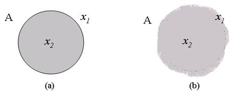
Figure 1a shows the situation exposed; element x 1 has a membership value equal to 0 since it is not included in set A, while element x 2 has a membership value equal to 1 since it belongs to set A. This is the fundamental property of conventional logic; the membership function can only have two values, 0 or 1. In the case of fuzzy sets, the situation is as shown in Figure 1b. Boundaries are not precisely defined; the degree of membership of an element can be any value between 0 and 1 between the membership of an element in a conventional set and a fuzzy set.
To understand the meaning of the membership function in fuzzy logic, now consider the following scenario. First, consider that the average temperature of the day is desired; whether it is cold temperature or warm, the limits are decided as follows:
Figure 2 shows the graphical representation of the relationships proposed in equation (2). Temperatures below 15 oC have membership grade 1 for the "Cold Day" set, and membership grades 0 for the "Mild Day" and "Hot Day" sets, and so on.
Now, consider the case where on a particular day, the average temperature is 14.95 oC; according to the definitions adopted, this day belongs to cold days. However, if the temperature were 15.01 oC, a difference of only 0.06 oC, the day would be considered mild. This, from a practical point of view, does not make much sense since the difference between the two temperatures is so tiny that it can only be appreciated using exact measuring instruments. In the absence of these, the definition of the type of day is imprecise.
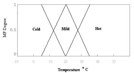
Figure 3 shows a possible graphical representation of fuzzy sets for the day's classification according to their temperature. In this case, the day is cold with a degree of membership if the temperature is less than 3 oC. The degree of membership to this set decreases linearly until it is 0 at 20 oC. Similarly, the degree of membership to the "Hot Day" set is defined as the degree of membership 0 to 20 oC, increasing linearly until it reaches 1 to 35 oC and remaining so for the rest of the temperatures. In the case of the set "Mild Day," the degree of membership is only 20 oC; for higher temperatures, the degree of membership decreases linearly to 0 to 35 oC. For temperatures less than 20 oC the behavior is symmetrical.
Consider now the case analyzed above, a day with an average temperature of 14.95 oC. Using Figure 3, it can be determined that for this temperature, there are three degrees of membership for this temperature, 0.32 for the set "Cold Day," 0.69 for the set "Mild Day," and 0 degrees for "Hot Day." These results coincide better with the assessment that would give anyone who does not live in Sahara; if you ask how, you would classify a day with this temperature; it is not a cold day; it is almost temperate. This is precisely the versatility of fuzzy logic; it allows mathematical expression of the vagueness and imprecision in the real world.
Definition of Fuzzy Set
First, it is necessary to define the universal set U as the set containing all possible elements, which has the characteristics to consider (Zadeh, 1965). The concept is equivalent to the concept of the universe used in Thermodynamics. Taking this concept into consideration, one can define a fuzzy set A in the universe U as the set of ordered pairs of a generic element and their degree of membership ( A (u), i.e.:
For practical purposes, it is the degree of membership that defines whether an element belongs to the fuzzy set and to what degree. For example, consider the set A of integers that are "near zero," then:
That is, -4 has a degree of membership 0 to this set, while 0 has a degree of membership 1 and 3 has a degree of membership 0.1, and so on for the rest of the elements.
Membership Function
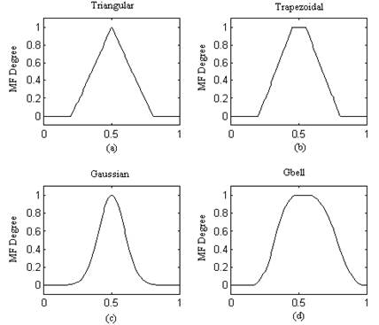
Membership functions are curves that allow you to determine the degree of belonging of an element u to a fuzzy set A. They are usually denoted by (, and their value is always between 0 and 1. Figure 4 shows the typically used membership functions:
The choice of the membership function to be used depends on the nature of the concept to be handled. For example, it is not the same to speak of "High Temperature" in an atomic reactor or an iron smelter as to do it when referring to a hot day. The final decision on the form of the membership functions to be used rests with the designer who analyzes the problem. However, triangular and trapezoidal membership functions commonly appear in the literature, possibly due to their simplicity.
Universe of Discourse
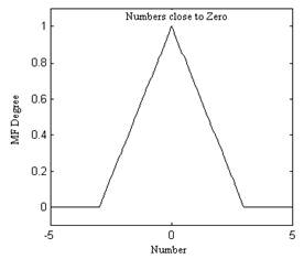
The universe of discourse is defined as the set of values that a variable can take. It is equivalent to the notion of the "domain" of a function. Figure 5 graphically depicts the fuzzy set of "numbers close to zero." In the graph, it is possible to observe that the universe of discourse for this case is the interval [-5,5]. The universe of discourse is always a conventional whole. Usually, the universe of discourse is denoted as E.
Operations with Fuzzy Sets
The following sections describe some of the essential operations and definitions related to fuzzy sets.
Operations with Fuzzy Sets
Let E be the Universe of Discourse to which the variable x belongs. Let A and B be fuzzy sets contained in E. Then A is said to be a subset of B if for any element x:
A is contained in B if the membership values of each element of x in A are less than or equal to its corresponding membership values in B.
For example, if you have the fuzzy sets A and B:
Then
The intersection of Fuzzy Sets
Let E the Universe of Discourse for the variable x, and let A and B be two fuzzy sets contained in E. The intersection of A with B is the most significant subset of E, which is at the same time part of A and also of B. The degree of membership of the intersection of A with B for each element is calculated as:
The degree of membership of the intersection of A with B is the minimum value between the membership values of each element in each fuzzy set. For example, If A and B are defined in E as:
Then
This could be seen in a graphic in Figure 6.
Union of Fuzzy Sets
Let A and B be two fuzzy sets contained in the discourse universe E, the union A(B is the smallest subset in E, including A and B. The degree of membership of each element x is determined in this case as:
In other words, the union is the contour that includes both sets A and B, resulting in a set larger than A or B. For example, If A and B are defined in E as:
Then
This could be seen in the graphic in Figure 7.
Complement of Fuzzy Sets
Let E be the Universe of Discourse of x, with the fuzzy set A contained in E. The complement of A concerning E is A', which contains the elements x contained in E, which are not members of A. The degree of membership of the add-in can be calculated as:
This could be visualized in Figure 8.
Overall Level
Let E be the Universe of Discourse of x. The set of elements of a fuzzy set A, with at least one degree of membership ( is called a level set ( or a cut set (. This definition can be expressed as:
Properties of operations of Fuzzy Sets
Given the discourse universe E and three fuzzy sets A, B, and C contained in E, the properties are shown in table 1 are satisfied. Moreover, most of the properties shown are identical for conventional sets:
Support of Fuzzy Sets
The support of a fuzzy set A, S(A) is the conventional set of all elements of the universe of discourse E. The membership function has a nonzero value.
Height of a Fuzzy Sets
The height of a fuzzy set A; hgt(A), is given by the supremum of the membership function for the entire Universe of Discourse E:
In this definition, the supremum refers to the largest possible degree of membership in the fuzzy set.
First expansion principle
In the description of many systems, different variables interrelate with each other using algebraic expressions and equations that reflect physical laws or properties of the system. For example, for an ideal gas, the expression:
Relates to all variables that affect the behavior of the gas. For example, suppose volume V is defined as a fuzzy set. In that case, it is desired to know how the pressure P will be affected and its behavior when V changes in terms of fuzzy sets.
In general, the question is: How to find the behavior in fuzzy terms of a variable, if its interrelation with another variable whose behavior in fuzzy terms is known?
The first principle of extension answers this question. Which states that:
Suppose one has a fuzzy set A, on the universal set U, and f is a mapping function from the universe U to the universal set Y, y=f(x). In that case, it can define a fuzzy set B in Y as:
Where:
The reason the supremum is used is that the function f can "map" different elements of the universe U into an element of the universe Y. Therefore, this element could have several degrees of belonging; hence it is necessary to choose a single degree of belonging, the supreme select among them the largest.
Fuzzy Numbers
Suppose the membership function support is part of the real axis. In that case, the fuzzy set represents a fuzzy number when the membership function is normal and convex.
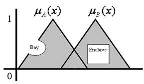
A membership function is regular if its height hgt is 1. In contrast, a membership function is considered convex if it does not assign more than one membership value to each element of its support. Geometrically this condition implies the non-existence of "bays" and/or "enclaves" in the contour of the membership function. Initially, its shape must be monotonically increasing, reaching a maximum value of 1, and then decrease, also monotonously or remain constant in this value if the trapezoidal type function is. Figure 9 shows nonconvex membership functions:
It is possible to define all arithmetic operations for fuzzy numbers. Similarly, fuzzy algebraic equations (Reznick, 1997), fuzzy differential equations have been defined, and the theory of stochastic phenomena has even been applied using fuzzy numbers (Liu, Heiner, & Yang, 2016). These works show that for every conventional mathematical operation, an equivalent operation can be defined using fuzzy numbers
Linguistic variables
A linguistic variable u in the universe of discourse E is defined as the set of linguistic value names T(u). Each value is a fuzzy number defined in E. For example, if u means speed, then in terms of its set, T(u) can be defined as:
In the universe of discourse E = [0,100]. Slow, medium, and fast are linguistic values of the linguistic velocity variable. Linguistic values accept qualifiers such as much, very, little, etc.. These qualifiers are used to increase linguistic values from a small collection of primary terms. For this purpose, processes known as intensification or concentration, dilation and defuzzification are used. For example, the very operator is defined as a concentration operator since, from the point of view of fuzzy logic:
Mathematical expressions that allow expressing qualifiers such as "very" or "enough" have been determined by some psychological experiments (Reznick, 1997). The mathematical forms commonly used to define them express the average opinion of a typical human expert. Of course, this implies that mathematical definitions by different authors may be different and that only common sense limits them. Nevertheless, authors such as Cox (2005) had classified the most commonly used qualifiers.
It is essential to mention that fuzzy qualifiers do not have a similar operator in conventional logic. Thus, for example, the linguistic terms very horizontal, very rectangular, etc., have no meaning.
Fuzzy Relations
The relationships between fuzzy sets and their application will now be considered, emulating an essential aspect of human thought: logical implication. This concept establishes the connections between cause and effect, or more formally, between a condition and its consequent.
In technical areas such as engineering or process control, these implications are present in almost any situation. For example, when a machine is operated, a process is modeled, or when a decision about purchasing equipment is made, etc., these decisions are based on logical implications.
Inference rules are usually used, as follows:
If Cause = A, then Effect = C
Where A and C set (fuzzy or conventional). For example:
If the level is high, then close the valve
In this case, the terms high and close represent fuzzy sets, high represents the linguistic value of the level variable. At the same time, close represents the linguistic value of the valve position variable.
There are much stricter definitions of fuzzy relations, which can be consulted in the literature (Reznick, 1997). However, with what has been described up to this point, it is enough to understand how fuzzy inference works intuitively.
Fuzzy logic-based controllers
Most conventional methods of controller design are based on the model of the process you want to control. Unfortunately, this implies at least two severe weaknesses. First, controllers are designed "tailored" to the process; the control strategy is designed only for the process that responds to the available model; if the conditions of the process change, the control strategy must be designed again. In addition, the time and effort involved in developing drivers for particular applications do not make them attractive from the practical point of view of the industry at large.
Second, for real complex processes, the model is often not known with enough precision to design a control strategy that is effective under all operating conditions.
A control strategy is then needed that does not require a process model based on the system's dynamic behavior and on the information that human experts have about the behavior of the process. Fuzzy logic emerges then as an alternative for the management of these systems.
Fuzzy logic-based control is a simple and easy-to-implement technology. It has the advantage of being very flexible and applicable to almost any system. The responses you get from the systems in which they are deployed are very smooth and very rarely reach unstable conditions. It allows incorporating the experience and knowledge that humans have about the process, who are in contact with it every day (Reznick, 1997).
The first to implement control based on fuzzy Logic was Mamdani (Harliana & Rahim, 2017), using a steam boiler and engine system as a process. Mamdani defined two input variables, the heat fed to the boiler and the opening of the valve that feeds the engine cylinder. In the same way, two output variables were defined: the pressure of the steam in the boiler and the engine's speed. This process presents a highly nonlinear behavior, the dynamics of the system changes with the point at which it is operating, so to implement linear control strategies, it is necessary to retune the controller whenever the point of operation of the process changes if you want to maintain a good performance of the control system.
Mamdani proposed to control the process using some fuzzy rules of involvement, such as:
If pressure error is Negative Large, Then the heat fed is Positive Large
The control strategy measured some process variables, applied some fuzzy rules, and determined the action to follow as necessary.
Mamdani designed his control strategy based on 24 fuzzy rules and using a PDP-8 computer. He also used a commercial digital controller as a comparison pattern. In all cases, the diffuse controller showed better performance than the digital controller, thus initiating a new era in process control (Reznick, 1997).
The basic structure of Mamdani Type Fuzzy Controller
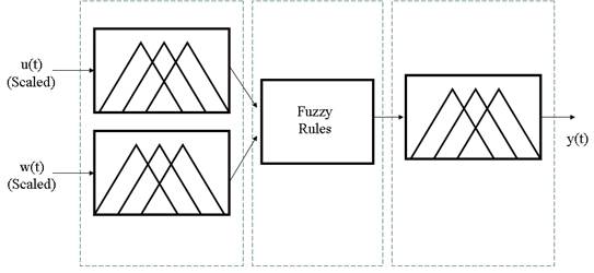
A Mamdani-type diffuse controller consists of three main blocks (Reznick, 1997):
Fuzzification Interface.
Fuzzy Processing.
Transformation to conventional value
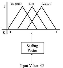
The fuzzification interface is responsible for converting the conventional values of the variables that enter the controller (error, variation of the error, etc.) into fuzzy values. It is necessary to remember that the signals that feed the controller come from a sensor, which sends readings proportional to the monitoring's physical variable. Therefore, they have a traditional value, not diffuse. Another aspect that needs to be considered in this conversion block is using a scaling factor to convert the actual input value into a value in the speech universe predicted by the designer.
Figure. 10 shows an outline of this process; the input is converted to an equivalent value on the scale of -1 to 1, then converted is the degree of belonging to each of the preset fuzzy numbers; 0.3 to Small Negative and 0.7 to Zero
The next stage is fuzzy processing. At this stage, fuzzy relationships that the designer establishes are used to decide what is convenient to take and keep the process under control. Fuzzy relationships, as mentioned in previous sections, have the form:
If Background then Consequent
The designer sets these rules based on his knowledge of the system and how he wants it to behave. This incorporates the human knowledge of an expert in the controller, giving it "intelligence" and flexibility.
Usually, when evaluating fuzzy input values, more than one rule comes into play, so the fuzzy processing result is a series of also fuzzy sets, the union of which gives the final result.
Figure 11 shows how the action to be taken by the controller is inferred from the values of the input variable; the fuzzy rules are applied, in this case, only two. Then the fuzzy sets obtained by applying the rules are joined, thus achieving the fuzzy value of the linguistic variable that defines the action to be taken by the controller
Since the evaluation of fuzzy inference rules is a fuzzy set, it is now necessary to convert it into a traditional value sent to the final control element. This operation is called defuzzification.
There are several methods to perform a transformation from fuzzy value to conventional value (Jang, Sun, & Mizutani, 1997), among them can be mentioned:
Centroid of Area
Bisector of Area
Media of Maximum
Takagi-Sugeno Fuzzy Modeling
Modeling by fuzzy identification receives great attention in nonlinear modeling, especially the Takagi-Sugeno (T-S) fuzzy model because of its ability to approximate any nonlinear model (Takagi & Sugeno, 1985). T-S fuzzy modeling has been used on nonlinear control systems (Herrera, Sarszosa, Paredes, & Camacho, 2019; Jiang, Gao, Shi, & Xu, 2010; Meda-Campana, Gomez-Mancilla, & Castillo-Toledo, 2012; Klug, Castelan, Leite, & Silva, 2015). The main idea of T-S fuzzy modeling is to approximate any nonlinear function by suitable linear subsystems.
An optimization method to improve the global approximation, local, and modeling capacity of the fuzzy T-S model is presented by (Al-Hadithi, Jiménez, & Matía, 2012). The main objective is to obtain an approximation of nonlinear functions with optimized performance. The basic idea in the estimation of parameters of the nonlinear system is to minimize a quadratic performance index, and it is based on the identification of the functions as follows:
Where for each IF-THEN  rule of a fuzzy system, in such a way that for a system of order n it can be rewritten as follows:
(24)
The fuzzy estimate of the output is given by
(25)
Where:
(26)
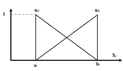
where 𝑢 𝑗 𝑖 𝑗 𝑥 are the different belonging functions which are assumed to be known to belong to the fuzzy set of 𝑀 𝑗 𝑖 𝑗 as represented in figure 12.
To start the identification methodology, for a set of input/output samples, 𝑥 1𝑘 , 𝑥 2𝑘 ,⋯, 𝑥 𝑛𝑘 , 𝑦 𝑘 , the parameters of the fuzzy model can be calculated by minimizing the performance index. A practical approach with a low computational cost is based on the parameter weighting method. The main objective is to improve the choice of the performance index and minimize it. This method is characterized by extending the objective function, including a weighting factor K and the norm of the vector P (Jiménez, Al-Hadithi, & Matía, 2008).
(27)
Where:
𝑌= 𝑦 1 𝑦 2 ⋯ 𝑦 𝑚 𝑡
𝑃= 𝑃 0 (1⋯1) 𝑃 1 (1⋯1) 𝑃 2 (1⋯1) ⋯ 𝑃 𝑛 (1⋯1) ⋯ 𝑃 0 ( 𝑟 1 ⋯ 𝑟 𝑛 ) ⋯ 𝑃 𝑛 ( 𝑟 1 ⋯ 𝑟 𝑛 ) 𝑡
𝑋= 𝛽 1 (1⋯1) 𝛽 1 (1⋯1) 𝑥 11 ⋯ 𝛽 1 (1⋯1) 𝑥 𝑛1 … 𝛽 1 ( 𝑟 1 ⋯ 𝑟 𝑛 ) ⋯ 𝛽 1 ( 𝑟 1 ⋯ 𝑟 𝑛 ) 𝑥 𝑛1 ⋮ 𝛽 𝑚 (1⋯1) 𝛽 𝑚 (1⋯1) 𝑥 1𝑚 ⋯ 𝛽 𝑚 (1⋯1) 𝑥 𝑛𝑚 …𝛽 𝑚 ( 𝑟 1 ⋯ 𝑟 𝑛 ) ⋯ 𝛽 𝑚 ( 𝑟 1 ⋯ 𝑟 𝑛 ) 𝑥 𝑛𝑚
And,
Equation 27 can be written as follows:
(28)
Applying the gradient operator and setting the equation to zero to minimize we obtain:
− X t Y+ X t X+K P=0
Thus, the parameters of the fuzzy model are given by:
(29)
where K is a diagonal matrix that must necessarily have nonzero values to guarantee that the term 𝑋 𝑡 𝑋+𝐾 is invertible.
Fuzzy PID Control
Process control plays an essential role in the safe manufacture of quality products; while there are several methods available to regulate this process, PID controllers have carried significant responsibilities due to its simplicity and reliability (Greg, 2000), however, being the PID is a linear controller is not well suited for strongly nonlinear systems (Yesil, Guzelkaya, & Eksin, 2003), for this reason, in the presence of complex nonlinearities and high uncertainties a fuzzy controller has emerged as a powerful tool to deal with such complex systems (Siddique, 2014).
In the work of (Mizumoto, 1995), the realization of the Fuzzy PID is presented; however, is the work of (Jantzen, 1998) that provides not only the structure of the Fuzzy PID controller but also a methodology to tune the aforementioned controller, which is used on this work with minor modification, and is presented as follows:
Tune the PID controller (any method)
Replace it with an equivalent linear fuzzy controller
Make the fuzzy controller nonlinear
As seen previously, the first step requires a classical PID controller tuned with any method (Ziegler Nichols, for example), providing the gains Kp, Ti, and Td of the controller.
The second step requires replacing the PID controller with the equivalent fuzzy controllers; this means, transform:
Into the following structure (Figure 12):
Where:
In case of being expressed with Kp, Ki y Kd:
To perform the replacement of the PID controller with the previous structure, certain considerations must be taken into account:
Universe of Discourse: The universe of discourse for inputs and outputs must be large enough to maintain the variables (error and control signals) between the boundaries (without saturation). Each input/output family must contain several terms, such as the sum of membership functions is 1 for each input/output.
Membership functions: Preferably use triangular membership functions that cross on (=0.5.
The number of rules: The number of terms on each family determines the number of rules, an AND connector is recommended combined with all terms to assure the completeness of the system, a rule of thumb to determine the number of rules that guarantees completeness is presented as follows:
Defuzzification method: Use the Centroid of Area (COA) method for defuzzification.
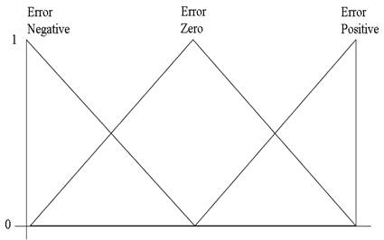
The final step requires to make the fuzzy controller nonlinear; in practice, a rule-based from terms like Positive Error, Negative Error, and Zero Error are commonly used as input family may consist of these terms, using (4) is possible to note that many applications only require nine rules of inference, specific rules could be omitted to modify the control surface (Jantzen, 1998). The shape of the rules are modified by replacing the triangular membership functions with Gaussian o Gbell type membership functions, also modifying GU, GIE, GE, and GCE, as various ways to reach the nonlinearity of this controller, but all this is done by experimentation adjusted to satisfy specific performance criteria
PID with Fuzzy Gain Scheduling
As stated previously, PID control is the most widely used control algorithm in the process industry; if specific performance criteria require dealing with strong nonlinearities, a Fuzzy PID is ideal for this application; however, if the traditional PID is combined with fuzzy systems into Gain Scheduling approach, the previously presented limitations of this controller could be overcome.
The first approach for Fuzzy Gain Scheduled PID was found by the authors of this work (Zhao, Tomizuka, & Isaka, 1993). The algorithm has been maintained through time practically with slight changes as found on Lisauskas & Rinkeviciene (2011), Bedoud, Ali-rachedi, Bahi, & Lakel (2015), and Qin, Sun, Hua, & Liu (2018).
The algorithm used in this paper is stated as follows: Consider a nonlinear plant regulated with a PID controller as presented on (1) with a prescribed universe of discourse for the error and error derivative signals  and
and  respectively, it is assumed that Kp, Ki, and Kd are in prescribed ranges; this is,
  ,
,  and
and  . Then, by using a Mamdani FIS, the parameters are determined by the following set of fuzzy rules:
Rule i=1,2,…..m
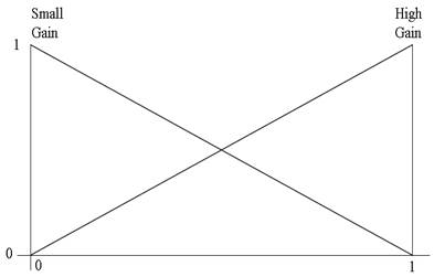
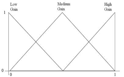
Where  is the membership functions used to describe the fuzzy inference systems. For instance, considers a set of triangular membership functions used to describe this system, a typical gain scheduler could be seen as follows (Figures 13,14,15):
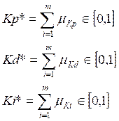
The defuzzification leads to the following:
The gains obtained on equation (5) are used in the calculation of the following normalized gains:
Finally, the block diagram of the PID with a Fuzzy gain scheduler can be seen in figure 16.
Fuzzy Adaptive MPC
A fuzzy adaptive model predictive control built on discrete-time is presented in this section; this approach was presented on (Aboukheir, Herrera, Chavez, Leica, & Camacho, 2020), firstly considers a nonlinear system with time delay and measured disturbances:
A persistent exciting input is introduced into the system in equation (36) to obtain a sufficient informative experiment for data modeling (Ljung 1999), assuming a sampling period T the following set of data  is obtained:
The Takagi Sugeno Model, including measurable disturbances, is the interpolator between linear ARMAX functions and ( ip the i-th memberships functions, presented as:
The defuzzified output  with (
ip
(((kT)) containing the information of all regressors, and (
i
the firing degree of th i-th rule:
Once the model is defined according to equation (38), the next step is the calculation of the corresponding predictive control law,
Definition #1: The cost function to be minimized by the predictive control law applied to the system presented equation (38) is defined as:
Where r(kT)  and u(kT) are the setpoint signal, the estimated output, and the control signal, respectively; finally, Hp is the prediction horizon. The control signal u(kT) is used instead of the classical MPC (u(kT) used in (Wang, 2009) as part of the modification proposed for the control algorithm.
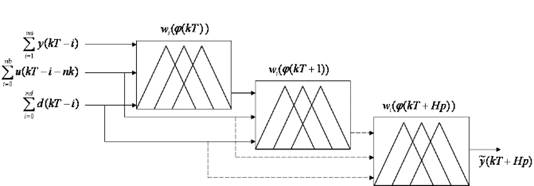
The first step on each control cycle is the prediction step, From j=1…Hp with Hp the Prediction Horizon, the proposed prediction vector on is built as follows:
This could be seen in graphic form in figure 17 for the generalized case as:
The prediction presented on equation (33) must be calculated for each sampling period, with the information provided by the fuzzy model on equation (31). This provides enough information for the Fuzzy MPC to guarantee a stabilizing control law overall operating regions.
With the information provided by the Hp Steps Predictor, the final step is the minimizations of equation (32); for this reason, consider the following theorem:
Theorem #1: The control law  that minimizes the cost function presented on equation (32) with the nonlinear system represented in equation (31) and predictions calculated according to equation (33) can be found by minimizing:
With
Where  used for prediction as presented in (33) and
  the control signal. Being a system under disturbances and time delay, a modification of equation (34) is used; this is, an adaptive penalization of the reference
  which is a function dependent on the disturbance above.
The proposed controller could be visualized in Figure 18.
Applications
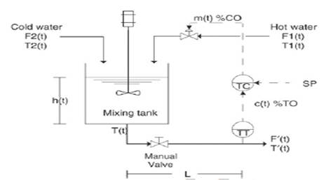
The mixing process presented in (Camacho & Smith, 2000) is used as a benchmark system to illustrate the design process of the previously presented controllers. Firstly, a hot water stream F 1 (t) (used as m(t) as control signal) is manipulated to mix with a cold-water stream F 2 (t) to obtain an output flow F 4 (t) at the desired temperature T 4 (t). The temperature transmitter is located at a distance L from the mixing tank bottom. This highly nonlinear system has the main characteristic of a variable time delay dependent on the fluctuations of F 1 (t) and F 2 (t); this process is shown in figure 19.
An equilibrium point must be selected to build a linear model; in this case, a First Order plus Dead time model or FOPDT for short. Consider, for instance, an equilibrium point m(t)=0.478, a disturbance signal of 15% of the value of the equilibrium point (m(t)=0.0717 is introduced, a set of FOPDT models are built, but the following model when W 1 (t)=125lbs/min is selected as the worst-case scenario (most significant disturbance):
The desired setpoint is T 4 (t)=150 ( F; a PID controller is designed for the model presented on equation (36), one possible configuration is presented as follows:
With:
With this in mind, the previously presented controllers are designed as follows:
Fuzzy PID Controller
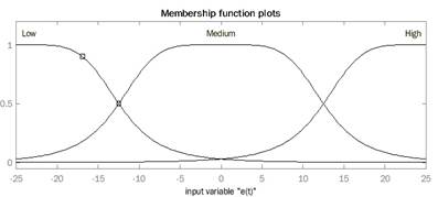
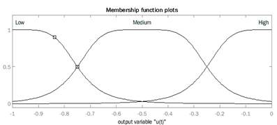
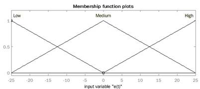
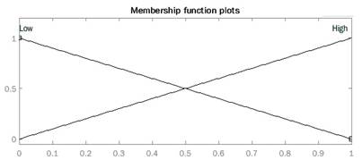
In this section, a Fuzzy PID controller is built following the previously presented steps; the first step defines the universe of discourse of  and u(t). Figures 20 and 21 illustrate the selected universe of discourse and the membership functions used; in this case, gbell mf are selected for this purpose
The next step is to transfer and upgrade the gains of the PID controller into the Fuzzy PID; as a rule of thumb, when using equation (25), it's possible to select the gain GU=-0.0001 this leads to:
With the selected gains, the inference rules are built, following equation (26) this leads to 9 rules which are presented as follows in table 2:
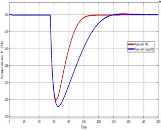
Figure 22 shows the performance of the closed-loop system with the Fuzzy PID against the PID controller.
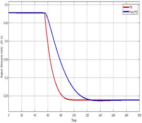
Figure 22: (a) Output of the system with (Red) PID (Blue) Fuzzy PID (b) Control Signal with (Red) PID (Blue) Fuzzy PID
As seen in figure 22, the fuzzy PID provides a softer response against the classical PID, both controllers perform well, if the control loop requires a softer response due to actuators restrictions, a fuzzy PID could satisfy this additional performance criterion of the systems
PID with Fuzzy Gain Scheduling
This section describes the procedure to build a PID with a fuzzy gain scheduler; the first step requires describing the universe of discourse for the inputs  and the outputs Kp, Ki, Kd. For the inputs, the Universe of Discourse previously presented is used in this case; however, the Universe of Discourse for the outputs must be described according to the desired performance criteria of the controller, in this case, a Reset Control approach (Barreiro & Baños, 2015) and (Bedoud et al., 2015). The reset control principle consists of resetting the integral (and derivative in this case) to zero every time the inputs (The error signals) cross to zero. The desired performance of the gain scheduler is established as follows:
The membership functions are shown on the following figures with its correspondent Universe of Discourse (Figures 23 and 24).
The set of rules are presented as follows in table 3:
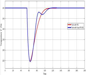
Finally, the performance of the closed-loop system with PID and PID with fuzzy gain scheduling is shown as upgrading the value of Ki=0.0014 (Figure 25), Figure 25b
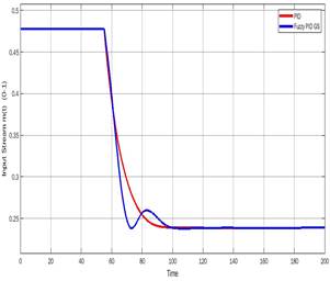
Figure 25: (a) Output of the system with (Red) PID (Blue) Fuzzy Gain Scheduled PID (b) Control Signal with (Red) PID (Blue) Fuzzy Gain Scheduled PID
As seen in the previous figures, the fuzzy Gain Scheduled PID recovers faster than the classical PID; however, when it is close to the setpoint, it reduces the effect of the integrator and derivation, providing a smoother approach to the reference; this type of controller is beneficial to avoid the windup effect that could appear on the classical PID controller.
Fuzzy Adaptive MPC
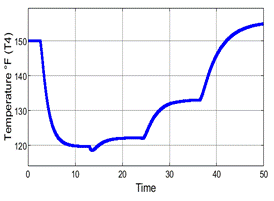
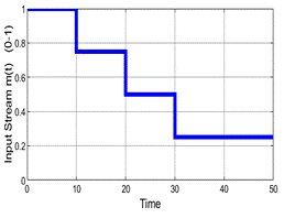
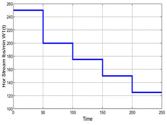
The FOPDT presented on (36) is no longer used on this part; instead of that, as stated in (Aboukheir et al., 2020), an experiment in the open-loop must be performed to obtain the input/output data to build the TS model presented on (31); first consider the Universe of Discourse [m(kT); W1(kT); T4(kT)]( UD with m(kT)([0,1]; W1(kT)([100,250] and T4(kT)( [118.6,154.9] with sampling period T=0.01 s, the following figures are obtained (Figure 26). Figure 26c, figure 26b
(a)
(b)
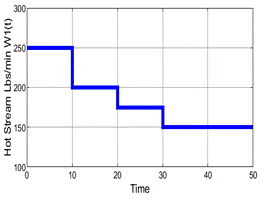
Figure 26: (a) Open Loop Output Signal T4(kT). (b) Open Loop Input Signal m(kT). (c)Measured Disturbance W1(kT)
According to (Aboukheir, 2010), a Fuzzy Takagi Sugeno first-order model under measured disturbances is selected; the proposed model is presented as follows:
With na=1 and nb=nd=nk=0.
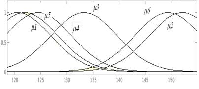
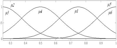
Using the sub clustering method (Abonyi, 2003) and gaussian type membership functions (Figure 27), figure 27b, figure 27c the proposed model in equation (41) approximates the measured output with an MSE < 10-6. Table 5 shows the rules used for this model:
(a)
(b)
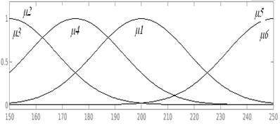
Figure27: (a) T4(kT-1) Memberships functions (iT4. (b) m(kT) Memberships functions (im. (c) W1(kT) Memberships functions (iW1
With this model in mind, the predictor is built according to equation (33) and, by selecting the penalization function , the following response against disturbance of the MPC controller is presented as follows:
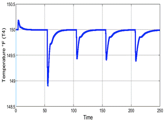
As seen in Figure 28a, the system follows the reference with great precision, rejecting the disturbance whenever they appear, as presented in Figure 28b.
Discussion
Each controller previously presented satisfy specific performance criteria; the effectiveness of each one relies on the specific requirements of the process and hardware available. For example, in the benchmark process previously presented, the Fuzzy MPC provides better disturbance rejection with practically no overshoot. However, some equipment installed on plant floors cannot handle this algorithm and must rely on the Fuzzy PID or the Fuzzy Gain scheduling. Which also provides good results respecting disturbance rejection and smoother control laws with less computation effort.
Finally, it is possible to conclude that a complete analysis of the process and a precise specification of its requirements, taking into account the restrictions presented (hardware, software, etc.) is the primary key for selecting the adequate control algorithm.
Conclusions
Fuzzy logic is a highly versatile artificial intelligence technique. It can be used successfully to model complex industrial processes and perform automatic control of them. The handling of this technique is very intuitive and can be learned very quickly. The process control applications in this article highlight the robustness of this technique. And how well it can be combined with other control techniques to achieve more stable and robust control systems than the originals.
The future of fuzzy logic in the field of process control is quite promising. Every day, new applications are reported in the literature, and new developments are seen that could be used daily by the industrial sector in the short term.
Conflicts of Interest
The authors must declare no conflicts of interest of any nature.
Contribuciones de los autores
En concordancia con la taxonomía establecida internacionalmente para la asignación de créditos a autores de artículos científicos (https://casrai.org/credit/). Los autores declaran sus contribuciones en la siguiente matriz:
Camacho, O.
Iglesias, E.
3.
Herrera, M.
Aboukheir, H.
Conceptualización
Análisis formal
Investigación
Metodología
Recursos
Validación
Redacción - revisión y edición


