Forma sugerida de citar:
Serrano, S., J. C. Ruiz and F. Bersosa. 2017. Heavy rainfall and temperature proyections in a climate change scenario over Quito, Ecuador. La Granja: Revista de Ciencias de la Vida. Vol. 25(1):16-32. pISSN:1390-3799; eISSN:1390-8596.
1 Introduction
The last report of the Intergovernmental Panel on Climate Change (IPCC AR5, 2014) indicated that there is a change in frequency and intensity of extreme weather events such as heat waves, intense precipitation, flooding, etc., in various regions of the world as a result of global climate change. These changes are particularly important for society and the environment, since by definition, they are outside the range of usual ecosystem adaptability, and thus can lead to severe impacts in biodiversity, agriculture, health infrastructure and economic losses (García et al., 2012).
Particularly, a general increase of temperature in Latin America was reported (Samaniego et al., 2009). It was also registered an increase in temperature of one tenth of a degree per decade over the Andes (Martínez et al., 2009); studies of Ecuadorian weather have shown that the temperature is gradually increasing over the region (Vuille et al., 2008; cited in Villacis et al., 2012). And studies have shown an increase of temperature in the four regions of Ecuador (Nieto et al., 2002; Cáceres, 1998). On the DMQ Zambrano-Barragán et al. (2010), and Villacis (2008), reveal an increase of annual temperature by 0.12°C per decade over a period of the last 100 years.
1.1 Extreme events indexes
In addition to the gradual behavior of a variable such as temperature, extreme events should also be recorded. The CCI / CLIVAR / JCOMM (Expert Team on Climate Change Detection and Indices) proposed a methodology which includes the RClimDex program for study extreme events in a climate change scenario (Karl et al., 1999; Peterson, 2001).
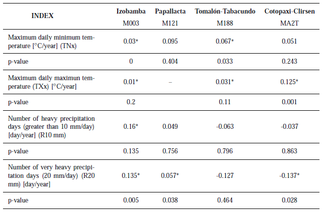
Thus, using RClimDex over the Metropolitan District of Quito DMQ, three possible threats related to climate change were identified: the extreme values of maximum and minimum daily temperatures all over the region, and the intensity of rainfall over the 90th percentile in the south and southwest of the DMQ. This analysis was constructed using available data from weather stations of INAMHI (Instituto Nacional de Meteorología e Hidrología de Ecuador) of the past 47-48 years (except station Tomalón-Tabacundo) with 21 years, located in four points of the District (Table 1). The trends are shown in Table 2.
When studying extreme values, it is necessary to change the statistical distribution because intense climate extreme events are more frequent than expected by normal distributions (Gilleland and Watts, 2005). The National Science Foundation (NSF) through the National Center for Atmospheric Research (NCAR), the Weather and Climate Impact Assessment Science Initiative, and the NCAR Geophysical Statistics Project (GSP), have recommended the use of the Extreme Value Theorem (EVT) and developed tools for the study of extreme weather events included in a specific software called eXtreme.
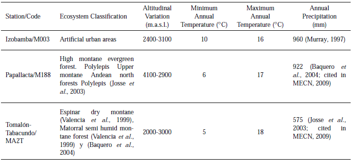
Table 1. Available weather stations with daily data selected for the study.† Cotopaxi-Clirsen station not presented continuous data.

Table 2. Annual trends of each R-Climdex indicator of climate change for extreme temperatures and precipitation for the four weather stations of DMQ and surroundings, ∗mean values with a significance superior to 90% (p<0.2).
1.2 Ecosystem description of the sample points
The DMQ is characterized by a great climatic and orographic variety, with the northwestern tropical, desert in the Guayllabamba Valley, the interandean permanently clouded forest in the cold mountain to urbanized city of Quito between the mountains that surround it. Giving as result a wide variety of ecosystems. However, due to the nature of the research, daily station data available only describe three types of ecosystems –with enough confidence–, which are presented in Table 3.
1.3 Generalized Extreme Value Distribution
Let X1, . . . ,Xn be a sequence of independent randomvariables, and let Mn = max{X1, . . . ,Xn} the maximum(or minimum) values measured on a regular timeline, so Mn represents the extreme values of the process in n time units of observation. For this data, and using a linear renormalization, the distribution of the set of Mn is given by the Generalized Extreme Value (GEV), which has the form:
where  and
and 
 are the parameters of location, scale and shape respectively (Coles, 2004).
This distribution depends on the sign of  if
if  we have the Weibull distribution, usually associated with temperature data if
  , we have the Gumbel distribution, and if
  it is a Fréchet distribution, commonly used to simulate the behavior of precipitation (García et al., 2012).
An advantage of GEVD is the possibility of a non-stationary model, allowing a time-dependent distribution by the parameter µ1 :
The parameter µ1 corresponds to the change of the location parameter, and could simulate the increasing or decreasing effects of climate change on weather variables.
1.4 Climate change models
In order to simulate the behavior of climate changein the planet, Global Circulation Models (GCM) were implemented by super computers, with horizontal resolutions of 300 km. In order to understand the behavior of the weather at smaller scales, there are Regional Climate Models (RCM), which work with scales of 50 km or less, allowing for more precise characteristics of the land surface and complicated mountainous topography, coastlines and the inclusion of small islands and peninsulas.
RCMs are very complete dynamic models, basedon the physics of the climate system, and virtually represent all processes, interactions and feedbacks between climate systems and the componentsof the GCMs (PRECIS, 2004).
An example is PRECIS (Providing Regional Climatesfor Impacts Studies), which is a regional climate modeling system developed by the Hadley Centre of the Met Office in the United Kingdom.It is a free software that allows the use of high resolution data in impact, vulnerability and adaptation studies as recommended by the United Nations Framework Convention on Climate Change (Articles4.1, 4.8 and 12.1).
PRECIS works with HadCM GCM model,which is forced by surface boundary conditionssuch as sea surface temperature and seaice fraction.It has two time periods: 1960-1990 a base timeor “control” period, used for comparisons withreal data; and 2000-2100, period used for forecasting.According to the IPCC (2001), circulation modelsare suggested to work with the A2 and B2 future scenarios agreeing to the economic and productive behavior of the planet and the possible incorporation of clean technologies. Where B2 scenario describes a world with a greater emphasis on local solutions to economic, social and environmental sustainability than A2. Both should be considerede qually right. The scenarios do not include additionalclimate initiatives. In this work, these two scenarios are used.
2 Materials and methods
2.1 DGVE, return levels and confidence intervals with real data
This study recorded maximum and minimum temperatures in four stations, which were the only availablein to DMQ with sufficient temporal range (morethan 30 years) and daily resolution; as shownin Table 1, their behavior and trends were calculatedusing R-Climdex (Serrano et al., 2012), and then used to calculate the climate change indexes shownin Table 2. With these outputs, and using the extReme software and DGVE functions, future behaviors were estimated of the maximum allowance for extremeevents of rain and temperature, with returnlevels for 2, 5, 10, 15 and 20 years and confidence intervals of 95%, for both A2 and B2 scenarios since 2012.
2.2 Fitting PRECIS data for each scenario
In order to determine the validity of PRECIS, itsgridded outputs for temperature, were used in the“control” period from 1960 to 1990 and comparedwith similar temporal periods for each station. A linearcorrelation for both the observed data and the modeled by PRECIS was made, finding the slope,the intersection in the middle of the series and thep-value for each case and achieving a correction factorby the difference in to the middle of the studiedseries (Table 4).
3 Results
3.1 Analysis of Maximum Temperatures by meteorological station
3.1.1 Izobamba
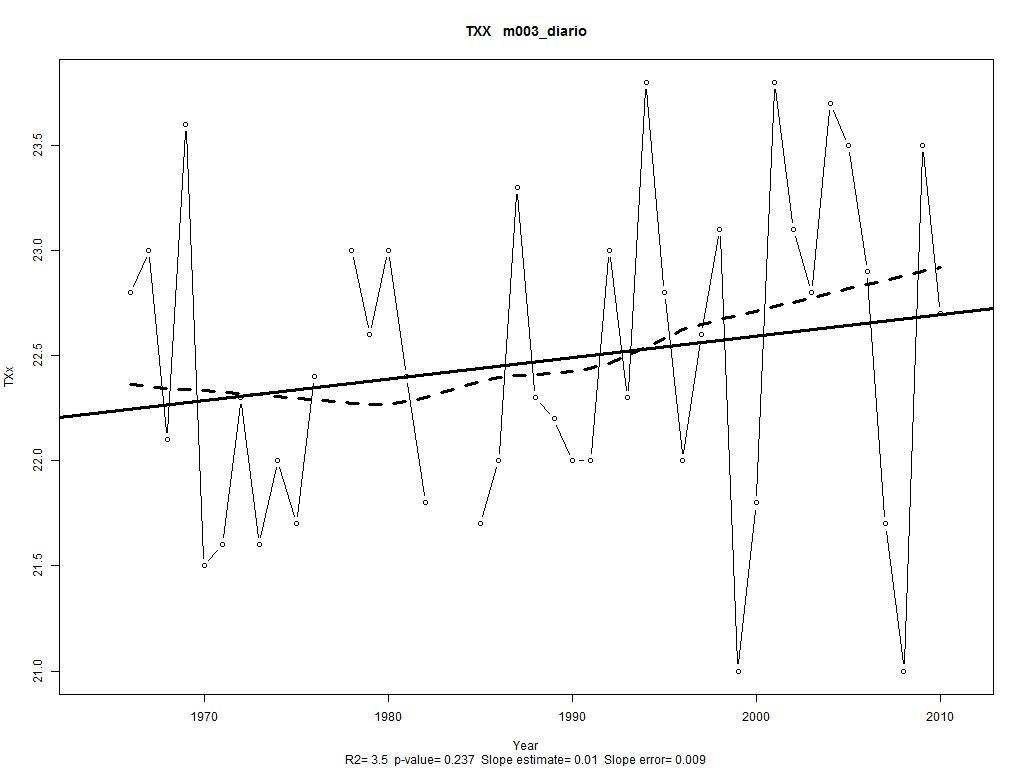
In Figure 1 the behavior of the maximum monthly value of the daily maximum temperature (TXX) in Izobamba, analysis achieved by R-ClimDex is shown. The trend of 0.01oC per year is statistically significant at 76.3% (Serrano et al., 2012).
Table 4. Correction factor by available meteorological station, between PRECIS time series and observed data, for temperature.

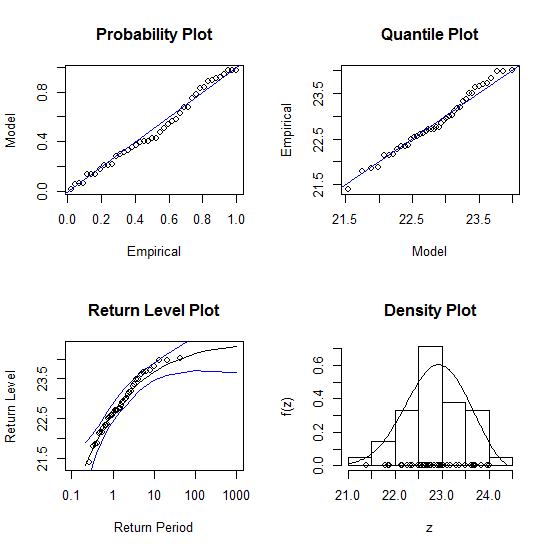
Figure 2. Adjusting of the maximum annual value of daily maximum temperature (TXX) in Izobamba for DGVE Weibull type distribution. The first two upper graphs show the proper fit of the model, while the lower left and right graphs show the return periods with confidence limits of 95% (blue line) and the probability density distribution.
Figure 2 shows the data set to a covariant DGVEwhere the results, after the maximum likelihood method, indicate that the location parameter variesover time like: μ= 22,65353(0,11592)+0,01t the scaleparameter is  0,65709(0,08777), and the shape parameter is
  −0,36045(0,14134), following a Weibull distribution. The maximum likelihood was 0.01303611, and the p-value has a significance value above 98%. Values in parentheses indicate the standard deviations of each parameter.
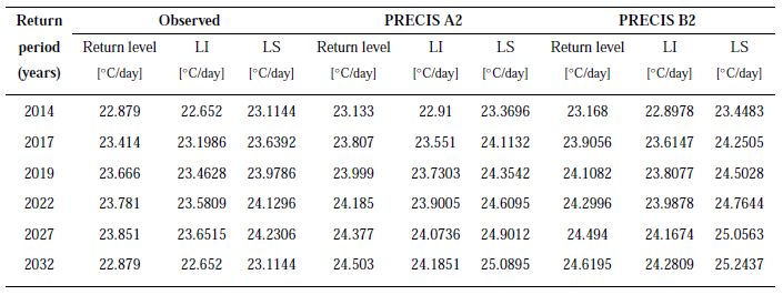
Return values and confidence limits for the Izobamba data studied up to 100 years are presentedin the lower part of Figure 2, but in detail,and for 2022 year are shown in Table 5.The value of the shape parameter for all periods is  −0,3604(−0,61849,−0,10241). Also, the settingsof trend data achieved with PRECIS for A2 and B2 scenarios are presented in Table 4 Thevalue of the shape parameter for all periods is
  −0,1751(−0,31983,0,02098) to A2; and
  −0,2264(−0,40246,−0,03666) to B2.
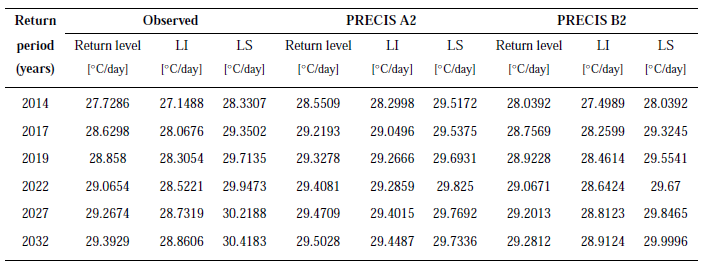
Table 5. Return periods, return levels and confidence intervals at 95% for the actual data of maximum temperatures in Izobamba.
3.1.2 Tomalón-Tabacundo
The same statistical treatment as performed to Izobamba was applied, and was recorded the highest slope of DMQ (0.125◦C / year) with a statistical significance of 0.999%. By simulating the data with acovariant DGVE the maximum likelihood method indicate a temporal variation of the location parameter: μ = 27,35713(0,29314)+0,125t, the scale parameter was  1,07630(0,21311), and the shapeparameterwas
 −0,33074(0,19109), showing that these data follow a Weibull distribution; the p-valuewas 0.1150664. The return levels and confidence limitsof the observed data and for the A2, B2 scenariosis presented in Table 6.
3.1.3 Papallacta
In the serie of the maximun value of maximun temperature there is a positive trend of 0.031◦C/year, with a statistical significance of 0.89%. The simulation a covariant DGVE and using the maximum likelihood method indicate that the location parameter varies over time as μ=19,39455(0,26281)+0,031t, the scale parameter  0,96090(0,19836), the shape parameter
  −0,28744(0,22732), showing that these data follow a Weibull distribution, thevalue-p-value 0.2363144, significant at 76% level. Comparison of return levels and confidence intervals for the two scenarios and the observed data ispresented in Table 7.
Table 7. Return periods, return levels and confidence intervals at 95% for analyzed data and both A2 and B2 scenarios of PRECIS for the next 20 years, for the maximum annual temperatures in Papallacta.
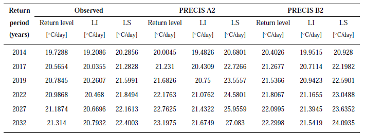
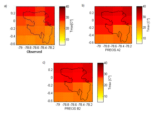
Figure 3. Maximum annual daily temperatures expected for the next 10 years in the DMQ in the color bar. Horizontal data shows the Longitude, Vertical the Latitude. a) forecast using the observed trend with real data from the studied meteorological stations, b) forecast using the product of dynamic forcing trend calculated by PRECIS A2 scenario c) Forecast using the product calculated by the dynamic forcing B2 (optimistic) scenario of PRECIS trend.
The GCM simulated data were regionalized using the technique of approaching averages, taking into account the annual mean temperature maps of the Ministry of Environment (MDMQ, 2011) and PRECIS model outputs, thus maps are presented with the resolution of this latter model. In Figure 3(a) shows the highest values of annual maximum temperatures that can be expected to 2032 year, these results take into account the dynamic forcing calculated by PRECIS scenarios A2 and B2, which are shown in Figure 3(b) and 3(c) respectively.
3.2 Analysis of daily minimum temperatures for Izobamba, Tomalón-Tabacundo y Papallacta
The behavior of the annual maximum values of minimum temperatures (early hours of dawn) for Izobamba station, located south of the DMQ is presented,into the series there is a positive trend of0.03◦C/year with a statistical significance of 75.7%.By simulating the data with a covariant DGVE,the location parameter was μ = 10,05092(0,13680)+0,03t, the scale parameterwas  0,78644(0,09780), and the shape parameter
  −0,22174(0,11901).Showing that these data follow a Weibull distribution.Also the test of maximum likelihood indicates that the p-value was 0,09103756.
In Tomalón-Tabacundo the trend was 0.051◦C/year, and the DGVE has a location parameterof μ=14,38173(0,29938)+0,051t, a scale parameter of  1,07082(0,23624), and a shape parameter of
  −0,27288(0,27655), in a Weibull distribution, the p-value was 0.3372716. Since in Papallacta, thetrend is positive too: 0.067◦C/year with a significanceof 96.7%. The return levels and confidence intervals for the two scenarios and the observed datafor the three stations for 2032 year is presented inTable 8.Similarly, the regional data of annual maximum values of minimum temperatures in the DMQ, forreal data and the A2, B2 scenarios are presented in Figure 4.
3.3 Behavior of the heavy rainfall in Izobamba, Tomalón-Tabacundo and Papallacta
The behavior of maximum annual values of maximum precipitation days (above the 95th percentile =20 mm/day) for Izobamba station, located south of the DMQ, shows a positive trend of 0.366 mm/year with a statistical significance of 96.7% (Figure 5).
However, in the case of precipitation, there was not detected a direct dynamic forcing producing its increase over time (IPCC, 2014), but the increase in extreme weather events in general. That is why we did not use PRECIS scenarios. Return levels and confidence intervals are calculated only with the observed data, as shown in Table 9.
By simulationg convariant DGVE results archieved after the maximum likelihood method in Izombamba, indicate that the location parameter varies µ = 52,16587(2,98138) + 0,366t, the scale parame- ter  17,45288(2,34374), the shape parameter
  0,18686(0,11512), showing that these data follow a Frechtel distribution with a p-value of 0.0622325. The results are shown in Table 9(a).
In Tomalón-Tabacundo, the dryest region,the maximun precipitation has a negative trendof -0.161 mm/year with a p-value of 0.649,the location parameter was chosen as μ =27,44210(2,31995), with a  8,65550(1,98911), and
  0,33574(0,22768), into a Frechtel distribution, the p-value was 0.02581635 (Table 9(b)).
In Papallacta there is another negative trend of-0.473 mm/yer (p-value of 0.211). The DGVE hasa location parameter of μ = 52,81604(7,64252),  34,79840(6,15202), and
  0,24224(0,14866), in aFrechtel distribution with a p-value of 0.03283383(Table 9(c)).
The regional data in Table 7 for maximum valueper year of heavy precipitation into DMQ is presentedin Figure 6.
4 Conclusions and discussion
4.1 Behavior of temperatures and ecosystemic impacts in the DMQ
In the DMQ were identified three types of threats related to climate change or climate variability: a statistically significant increase in the magnitude of both maximum and minimum temperatures and an increase in the frequency of heavy rainy days (Serrano et al., 2012).
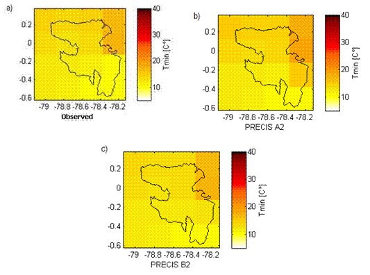
Figure 4. Annual maximum of daily Minimum Temperatures expected for 2032 year in the color bar. Horizontal data shows the Longitude, Vertical the Latitude. a) forecast using the observed trend of real data from the meteorological stations, b) forecast using the product of dynamic forcing trend calculated by the A2 scenario PRECIS, c) forecast using the trend product calculated by the dynamic forcing B2 scenario of PRECIS.
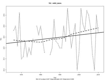
Figure 5. Annual behavior of the daily maximum precipitation values recorded since 1964 in the year 2011 in Izobamba.
Table 8. . Return periods, return levels and confidence intervals at 95% for both scenarios A2 and B2 of PRECIS for the next 20 years, for the minimum annual temperatures in a) Izobamba b) Tomalón-Tabacundo c) Papallacta.
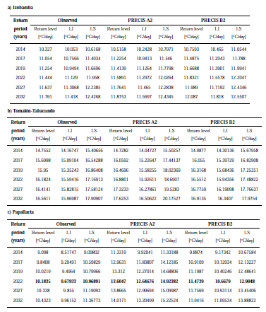
Table 9. Return periods, return levels and confidence intervals at 95% for the actual data of maximum heavy rainfall in a) Izobamba, b) Tomalón-Tabacundo, c) Papallacta.
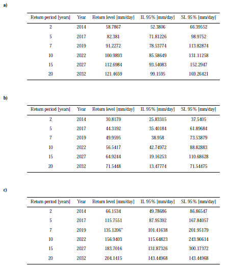
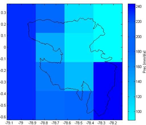
Figure 6. Possible values of maximum daily precipitation forecasts for the next 10 years in the DMQ year in the color bar. Horizontal data shows the Longitude, Vertical the Latitude. The figure shows the values of extreme events by day expected during this period, since Table 7.
The first part of this study, was aimed to know the intensity of extreme events of the minimum and maximum temperatures in the near future (2032 year), using DGVE distributions which indicated that the best fit to the temperature values was given by a Weibull covariant distribution i.e. involving a forcing behavior data. Thus, we have worked with the atmospheric forcing presented in PRECIS for A1 and B1 scenarios. In consequence, this study used both: a dynamic and statistical prediction.
Results show that for 2032 year, in the southernarea (Izobamba), where the average daily maximumtemperature is 14.6◦C, it will be possible observeextreme events such as temperatures up to23.7◦C, and according to the A2 and B2 scenariostemperatures as high as 24.3◦C and 24.2◦C respectivelycould be observed, i.e. an eventual increaseof about 10◦ over the average. It is expected to occurin the months of August and September, whichcorresponding to the dry season in Quito.
In the southeastern region (Papallacta) wherethe average daily maximum temperature is 14.4◦C,it is expected to register extreme events of 21◦C, andaccording to the A2 and B2 models 21.8◦C and 21.1 respectively, about 7◦C above average temperature.While in the north-east, the warmest region in DMQ, averaging 21.6◦C, in 10 years it is possible tofind extreme values up to 29◦C and using the A2 and B2 scenarios of 29.4◦C, and 29◦C respectively,i.e. 8◦C more than average.
In the case of minimum temperatures, in Izobamba whose average daily minimum temperatures are 6◦C, is expected to record extreme eventsof 11.4◦C, 11.6◦C and 11.8◦C according to statisticaldata and scenarios A2 and B2 respectively, anincrease of nearly 7◦. In Papallacta, with an average lowest temperature of 5.5◦C, it is expected to have extreme temperatures as low as 10.1◦C and A2 and B2 respectively 13.6◦C and 11.4◦C models, anincrease of more than 8◦C. Also, in the warmest region of the DMQ, where station Tabacundo Tomalonis located, has an average of 9.11◦C, and the modelcan be registered 16.2◦C, 16.8◦C and 16.5◦C accordingto statistical trend and the two scenarios A2 and B2, i.e. more than 7◦C for the next 10 years.
It should be noted that these values are possibleextreme temperature events, whose frequencyis casual, but the intensity has been shown to consistently rise may experience extreme events between 6 and 10◦C more than average temperaturesto which ecosystems are already accustomed.
4.2 Behavior of heavy precipitation
In the case of the precipitation DGVE indicate that the better option is to use a no covariant Fretchel distribution. In Izobamba, registered as the rainiest region, with a mean daily rainfall of 6.8 mm, it is ex- pected to register single events to up 100 mm/day, 14 times more than the average. The southeastern area represented by Papallacta has daily rainfall averages 3.7 mm/day, and in the next 10 years may register 156 mm/day, i.e. 42 times more. This phenomena occurs because Papallacta has historically registered record rainfall of 183 mm/day and 160 mm/day on 27 and 25 March 2003 respectively. Therefore it is very likely that the coming years will see a similar events of this magnitude.
As for the northeast, where the station Tomalon-Tabacundo is located, average rainfall of 4.3 mm/day and can record maximum of 56.5 mm/day are recorded. It should be noted that in this area the rains are often scarce, and there is a tendency to decrease precipitation and hence the hardening of dry regime.
4.3 Ecosystem impact
Because the DMQ have varied ecosystems with well defined characteristics, it becomes clear that these areas are affected differently.
On what it refers to the increase in minimum temperatures, even though it is a measure generally taken in the early hours of the morning, it is a direct measuring of warm nights. And it would be an in- dicator of potentially harmful effects by the lack of night cooling and main contributor of heat stress in animals and plants, especially those located in the transition zone of the paramo and are not adapted to these conditions. Also, it is noted that besides the presence of greenhouse gases that increase night time temperatures, must be added the heat island effect, which must be taken into account in all sampling points, as the effects urbanization resulting inincreased heat released during the night by modernin rastructure.
The increase in maximum temperatures, usually achieved at noon, directly affecting the adaptability of animal and plant species, including humans; because in a context of physical stress, coupled with high temperatures can be triggered death. Also, this indicator can also be interpreted as a measure of greater or lesser heliophany cloud cover, which can also favor the drought (Frich, 1999).
Also in the context of climate change, greenhouse gases favor the hydrological cycle and collaborating nucleation of water vapor into rain. While the increase of temperature favors the greatest amount of water vapor available, and hence is generated more intense precipitation. Those ecosystems that have more absorbency due to its vegetation cover would not be as affected by these sporadic events, although the edges urbanized city located in areas at risk by land slides are. Furthermore, it is noted that in the dry Northeast of DMQ has identified a negative trend in the presence of rain, which could result in the tightening of dry conditions in the area, affecting mainly to their biodiversity (Riebeek, 2005).
On the behavior of disease vectors, investigations of Rodriguez and Buitrón (20014) had been established that the increase of temperature and humidity favors the occurrence of diseases produced by insect vectors such as Anopheles mosquitoes and Aedes, responsible for the transmission of malaria and dengue. It was reported in 2010, in the provinces of Carchi (300- 4.723 m.a.s.l.) and Imbabura (1200 a 3000 m.a.s.l.) seven cases of dengue fever were confirmed, since National Institute of Hygiene Izquieta Perez (INHIP). Aedes currently aegypti is able to survive between 1,500 and 1,700 meter, meanwhile Varsovia Cevallos (El Comercio, 2010) conclude that under certain conditions of microclimate the mosquito could adapt to Quito and therefore could be cases of dengue, as happened in Galapagos in 2002 where the disease first and then the vector was reported. Ramirez et al. (2009), estimated that 34% of the world population would be at risk of contracting dengue. In Ecuador 70% of its territory is favorable for the presence of Aedes aegypti.


