1. Introduction

Ecuador is a country located in South America just in the middle of both hemispheres. Because of its location, near the Pacific Ocean, between the Andes Mountains, and next to the Amazon, this country has three natural regions: Coast, Highlands and Amazon (^{Iriondo, 1994}). This characteristic has allowed that the country has many exportation goods, being known by its agricultural products such as banana, roses and sugarcane, that are continuously increasing their exportation (Banco Central del Ecuador, 2017). Between 2013 and 2016, production and harvested area of sugarcane increased by 21% and 4% respectively (Corporación Financiera Nacional, 2017). Many zones in Ecuador have the ideal conditions for the sugarcane growth, this is the case of the limit between the Highlands and the Coast, where the weather is warm and the humidity allows the adaptation of the sugarcane. Places near the Highlands have an ideal climatic conditions to growth of this crop, this is the case of Nanegalito, a rural parish of Quito, located just in this limit, in the foothills of the Andes Cordillera, with a mountainous relief with slopes between 15 and 30 %, heights between 1400 to 2800 m, and with a humid climate with temperatures between 15-22 °C (Sistema Nacional de Información, 2017). The economy is principally based on agriculture and livestock, where more than the 35 % of the population works. Due to the presence of slopes, the presence of rains, in this location, it could increase the risk of soil erosion. Additionally, the lack of rains could also affect to the normal growth of the crops. In this way, some tools are useful to take advantage of the climatic information, among them it is found the typical meteorological year (TMY). In the beginnings, this tool was a set of numerical values of hourly radiation that corresponding to an hypothetic year that is constructed by choosing, for each month, a real year, that each mean monthly value of the global irradiation, be representative for all the years (^{Lerum, 2008}). Nowadays, this approach is employed to estimate the annual energy consumptions of buildings (^{Jiang, 2010}).

The most used method for calculate the TMY is the Finkelstein-Schafer statistical method, and during the years, different studies have been developed in order to measure the TMY in many countries for renewable energies e.g. Argentine (^{Bre & Fachinotti, 2016}), Turkey (^{Pusat, Ekmekçi, & Akkoyunlu, 2015}), India (^{Murphy, 2017}), Nigeria (^{Ohunakin, Adaramola, Oyewola, & Fagbenle, 2013}). Moreover, the TMY has been adapted to improve the agriculture in the garlic growing (^{Domínguez et al., 2013}), and optimize the irrigation water distribution through the crop cycle (^{Leite, Martínez-Romero, Tarjuelo, & Domínguez, 2015}). In this context, the TMY is helpful to determine the representative conditions over a long time period (^{Marion & Urban, 1995}), and also could be used as a tool for some decisions on agriculture as was pointed above.

In this framework, the aim of the present work was to determine the TMY in a function of precipitation for Nanegalito by the Finkelstein-Schafer statistical method from 12 years data. The approximation of the calculus made for Nanegalito could be used to a near parish such as Pacto, with the same altitude, crops and climatic characteristics, where there is no any weather station.

2. Methodology

The weather station of Nanegalito (M0339) reports only precipitation data, and is located in the UTM coordinates 757781 E y 10007068 N. The main climate in Nanegalito is a Subhumid Climate, Mesothermal hot tempered (Instituto Nacional de Meteorología e Hidrología, 2017). The precipitation data was taken from daily data from 12 years in the period of 2004-2015, with a total of 4300 data approximately. This data was obtained from the “Instituto Nacional de Meteorología e Hidrología” (INAMHI) of Ecuador. Fortunately, the database taken was complete, i.e. there was no need to complete missing data.

The method used in the present work was the Sandia Revised Method (^{Hall, Praire, Anderson, & Boes, 1978}), which is employed to determine the TMY of a location. In order to accomplish the requirements, were selected the data with ten (10) or more years of consecutive measurements (^{Janjai & Deeyai, 2009}). The data selected provided continuous data without missing information, which was helpful for the calculations.

The initial step was to collect the data from Nanegalito weather station (M339). With this data, 12 years from 2004-2015, the TMY was computed. Figure 1 shows the location of the Nanegalito weather station in the Province of Pichincha.

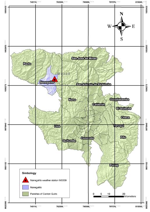
Figure. 1: Location of Nanegalito weather station in the Canton of Quito of the Province of Pichincha. 

The first step was to obtain the specific ranges and then establish the cumulative distribution function (CDF) for each month of the precipitation parameter, for the 12 years period of Nanegalito (2004-2015). Next, with the CDF data, the Finkelstein-Schafer statistical equation (^{Jiang, 2010}) was applied (Equation 1).

(1)

Where, N is the daily measurements in the month, CDF_m is the long term (12 years in this study) and CDF_y,m (for each year) is the short term cumulative distribution function.

With the calculated FS values, the weighting factor for precipitation was applied in order to obtain the Weighted Sum (WS) showed in Equation 2.

(2)

Where, M is the number of considered meteorological parameters, in this study was only one, precipitation. WF_x is the weighting factor of precipitation, and FS_x is the value obtained. Table 1 shows the weighting factor used in this study (^{Oko & Ogoloma, 2011}).

Table 1 Weighting factors for TMY (^{Oko & Ogoloma, 2011}). 

Tmax=maximum temperature, Tmin=minimum temperature, Tavg=average temperature, RHmax=maximum relative humidity, RHmin=minimum relative humidity, RHavg=average relative humidity, W=wind, Sd=sunshine hours, RF=rainfall, Evap=evaporation, G=global solar radiation.

Afterward, in order to select the typical meteorological months (TMM), that are employed to build the TMY, five candidates with the lowest WS were chosen. Finally, the root mean standard deviation (RMSD) was adapted to the precipitation, a simply method developed by ^{Pissimanis et al. (1988}) to select the TMM (Equation 3). Where, is the rainfall measured during each year, month and day of each candidate, is the rainfall average of the long period.

(3)

3. Results and discussion

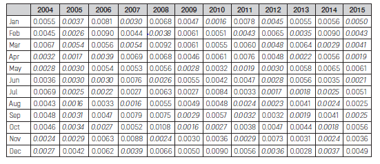
First, the CDF is calculated for each daily variable, in this case precipitation, in order to calculate the FS values, through Equation 1. The FS values for each month of each year is estimated and shown in Table 2.

Table 2 FS values of precipitation for Nanegalito station. 

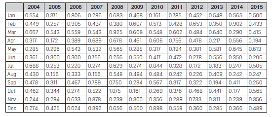
Second, the WS values were calculated through Equation 2, and were selected five candidates, which corresponding to the lowest values, that are shown in cursives in Table 3.

Table 3 WS values, cursives and underlined show the five lowest values.  

Consequently, the selection of the typical meteorological moths (TMM) is done using the Equation 3, with the RMSD, from the five candidates per month, observed in the Table 3. Thus, the typical meteorological year (TMY) is constructed from the values chosen, as seen in Table 4.

Table 4 TMY selection of Nanegalito station 

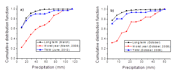
Moreover, the CDF values obtained from the long term (12 years), the highest WS value (worst year), and the TMM selected by RMSD (ideal year) are compared. The Figure 3 shows, illustrate as an example, the CDF values, with the previous considerations, of June (Figure 2a) and October (Figure 2b).

Both figures show that the CDF values of the TMM selected are similar to the CDF values of the long term, in contrast to the CDF values of the worst year (2008). Similar behavior have been reported by ^{Jiang (2010}) and ^{Bre & Fachinotti (2016}) who reported a TMY for China and Argentine.

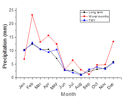
Additionally, the selected TMY is compared with the average of each month in the long term evaluated, and the worst months, Figure 3. It could be seen that the difference between the selected TMY and the long term average is lower than the difference between the worst months and the long term average. The higher precipitation values are seen in the rainy season (Oct-May), and the lower values are in the dry season (Jun-Sep). This trend does not change during all three curves analyzed. Similar results were observed by other researchers that reported analogous behaviors by comparing global radiation, wind speed and temperature (^{Bre & Fachinotti, 2016}; ^{Jiang, 2010}; ^{Pusat et al., 2015}).

Figure. 3: Comparison of the annual variation of the long term versus the worst year and the TMY selected. 

4. Conclusions and recommendations

The present work determined the typical meteorological year (TMY) of Nanegalito from precipitation daily values. The period considered was 12 years from 2004 to 2015, included both years. The Finkelstein-Schafer statistical equation was considered to calculate the TMY.

The results indicate that the Finkelstein-Schafer statistical equation is adequate to determine the representative months of the precipitation parameter in Nanegalito parish.

The CDF obtained shows a small difference between the selected TMM and the global years, expressed as long term.

The TMY computed express a suitable description of the months that better represents the climate, of the period analyzed, of Nanegalito parish.

The establishment of the TMY in Nanegalito, could be used in Pacto, and is a good management tool to contribute to the development of plans for prevent possible risks of drought in different crops such as sugar cane. The development of the TMY for more meteorological parameters could be useful to contribute to the management of renewable energies.