1. Introduction
In recent years, different air pollution events have called the attention of experts both in academic and government (Li, Fan, and Mao, 2016). According to Kim, Choi, and Kim (2005) in mega-scale metropolitan cities, the ozone pollution, has often been treated as one of the most serious socio-economic issues due to the frequent warnings associated with ozone exceedance episodes. Air pollution is any substance which may harm humans, animals, vegetation or material (Kampa and Castanas, 2008). Air pollutant levels even below standard concentrations are known to affect human health, with increases in respiratory symptoms, chronic cough, bronchitis and chest illness, also deterioration in pulmonary function (Fukuda, 2007). According to Katz (1970), a significant number of industrial activities contribute thousands of pollutants to the atmosphere. For that reason, environmental managers and urban planners seek monitoring and controlling levels of air pollution to make the decisions which allow mitigating health and the environmental risks.
Air pollution is monitored by stations, which generate data about levels of concentration of air pollutants in a specific zone. Data that is essential to properly evaluate air quality. However, many of these pollutants react chemically or photo chemically to produce new reactants (Katz, 1970). Therefore, information about associations among air pollutants, it is of great importance to support such evaluation. In this context, Cagliero et al., (2016) claim that the combinations of pollutants that simultaneously exceed the critical level, in most cases are particularly interesting.
Efficient air pollution evaluation requires well-grounded knowledge concerning emission sources, associations among air pollutants and their effect on air quality (Wagner, 1994). For this reason, countries from the Andean region as Ecuador search to improve their process to the discovery of knowledge in their environmental context. Hence, there is a need for effective strategies to extract knowledge from these datasets. In this context, data mining is a useful and flexible tool for knowledge discovery in environmental systems (Fukuda, 2007). Thus, we raise the following problem: how to use data mining techniques to identify associations patterns among common air pollutants in the Andean region? To address this problem, we developed an approach for discovery of knowledge based on a Cross-industry Standard Process for Data Mining (CRISP-DM) (Wirth, 2000). Unlike related jobs (Cagliero et al., 2016; Doreswamy and Manjaunath, 2015; Kingsy et al., 2016), this approach by means of Time Rolling Correlations leads to identify behavioral patterns among five harmful air pollutants in the Andean region: Ozone (O3), Carbon monoxide (CO), Sulfur dioxide (SO2), Nitrogen dioxide (NO2) and, Particle material (PM2.5). Correlations among pollutant levels can vary over time and space. Therefore, users are commonly interested in monitoring their temporal and spatial evolution (Cagliero et al., 2016).
This approach aims to support environmental managers to produce knowledge about air pollution. We claim that the proposed approach generates correlations that can assist environmental managers and urban planners in the decision-making process and consequently improve the life quality of citizens. We hypothesize that the application of data mining techniques helps identifying patterns of behavior among several air pollutants. To evaluate the implementation of the proposed approach, we use a real air pollutants dataset from Cuenca, Ecuador. This paper is organized as follows: in Section 2, we address the general background and related work. In Section 3, we detail the Data Mining approach. In Section 4, we describe the proposed approach experimentation. Finally, in Section 5 we present conclusions and future work.
2. Background and related work
According to Wirth (2000), data mining process needs a standard approach which helps to translate business problems in data mining tasks, suggest appropriate data transformations and data mining techniques and, provide significate information for evaluating the effectiveness of the results and documenting the experience. Cross-industry standard process for data mining (CRISP-DM) is a model for carrying out data mining projects processes (Wirth, 2000).
CRISP-DM is composed of six phases: business understanding, data understanding, data preparation, modeling, evaluation and, deployment. These phases have frequent dependence since they represent the life cycle of a data mining project (Wirth, 2000). Business understanding is focused on project objectives and requirements from a business perspective. Data understanding is focused on knowing the data and to discover first insights. Data preparation covers activities to construct the final dataset. Modeling is focused on select and applied modeling techniques. Some techniques require specific data formats. Therefore, there is a close link between Data Preparation and Modeling. Evaluation is focused in reviewing the steps executed to construct the model to be certain it properly achieves the business objectives. Deployment is focused on representing the knowledge gained in a way that the customer can use it (Wirth, 2000). This paper summarizes CRISP-DM phases in four stages.
In the modeling phase, there are several data mining techniques which can be applied according to the problem to solve. Algorithms oriented to the grouping of data, as well as, techniques for treatment and data analysis are addressed to follow.
Grouping algorithms
Data grouping algorithms divide a dataset into groups with some similarity. This paper is focused on the use of X-means and K-means grouping algorithms. X-means find the efficient cluster number among a maximum and minimum values. This algorithm uses the KD-Tree technique to improve the speed. X-means is composed of two steps: Improve-Params and Improve-Structure. The first step applies K-means to get k in convergence starting from k equal to the minimum value provided. The second step begins by dividing the center of each group into two branches in opposite directions along a random vector. If k> = k (max) the processing ends and reports the model with the best score (Kumar and Wasan, 2010).
K-means takes a dataset X = {x1, x2, ..., xm} and divides it into k groups. This algorithm groups data points by average values using the Euclidean Distance obtaining C = {C1, C2, ..., Ck}, so that, while less similarity there are among the classes, greater similarity there is among elements from a class (Zhang, Deng, and Li, 2017).
Techniques for treatment and data analysis
Techniques for processing and data analysis allows us to work with data in different measurement units. This paper is focused on the use of the correlation matrix technique, as well as, on the process "Select by weights" use. The correlation matrix is a symmetric matrix of n x n for n vectors. Each position (i, j) has a value between 1 and -1, such position is the value of the Pearson correlation (Gao, Tung, and Yang, 2017). The "Select by weights process" selects only those attributes from an input "ExampleSet" whose weights satisfy the specified criterion for the input weights. Input weights are provided through an input port. The criterion for selecting attributes by weight is determined by a weight relation parameter («Select by Weights - RapidMiner Documentation», s. f.).
In the air pollution context, both algorithms and data mining techniques have been examined in the literature from three perspectives: pollutants predictions, infrastructure improvement, and correlation analysis. Du and Varde (2016, p. 2) use data mining algorithms for association, grouping and, classification to identify correlations among PM2.5 pollution and traffic, in order to make predictions of PM2.5. Souza and Rabelo (2015) applied association rules to find correlations among air pollutants and respiratory problems. Shazan et al., (2017) use a spatial data mining technique to find associations between spatial features. Such research seeks to analyze whether the maternal exposure to air pollutants during pregnancy could be potentially associated with adverse birth outcomes (Shazan et al., 2017).
The literature reflects the use of data mining in air pollution studies. However, research focused on data mining to analyze the correlation between several air pollutants as O3, CO, SO2, NO2, and PM2.5 is scarce. Such analysis is essential to provide complete information to support the decision-making process of environmental managers and urban planners.
3. Data mining approach to identify behavioral patterns among air pollutants
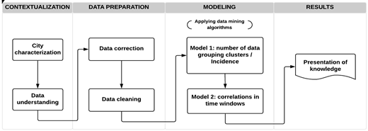
Based on CRISP-DM, the approach proposed in this study is divided into four stages: contextualization, data preparation, modeling and, results. Figure 1, shows the proposed approach flowchart.
The stages are composed of procedures which lead to the identification of associations among air pollutants. Results are presented considering elements of temporality. The following sections present in detail every stage.
Contextualization stage
Generally, data is captured by time intervals in seconds or minutes, according to the sensor configuration, and stored in databases. However, cities have specific characteristics according to its localization, so that the monitoring of air pollutants can change from one country to another. Consequently, this stage aims to promote a first contact with the data. In this paper, the proposed approach focuses on five air pollution elements: O3, CO, SO2, NO2 and, PM2.5.
Data preparation stage
The data preparation stage focuses on two procedures on a dataset to get a “valid” data input before the analysis process: data correction and data cleaning. The data correction procedure seeks to get real data values from location. In the case of data correction, the literature suggests using the barometric pressure and the temperature of the locality to be analyzed. For that, generally, it is applied the formula in Equation 1 (Walden and Andrew, 2013).
Where: Cc: Corrected concentration, Co: Observed concentration, Plb: Pressure local barometric (millimeters per mercury), tC: Local temperature (degrees centigrade). The data cleaning procedure seeks to obtain a clean sample for the study. For that, this paper proposes to manage the data through the next steps. First, obtain a row for a time interval for all pollutants. Second, control the null values normally generated by problems in the calibration of the sensors, the process may result in: impute with learning algorithms, replace with means if the dataset has a normal distribution or delete null values if the null values subset is short. Third, obtain samples with all-time interval records, this step consists of obtaining samples of days with complete records. We suggest filtering the days with the total of records greater than 99% due to the sensors could fail and do not record all times intervals on a day.
Modeling stage
The purpose of this stage is to create models to group techniques and algorithms for the data mining in air pollution context. Thus, we propose two models for data processing which are composed mainly of two algorithms: X-means and K-means. For the correct operation of these algorithms, the dataset requires only numeric values. Therefore, the data preparation process must be applied beforehand.
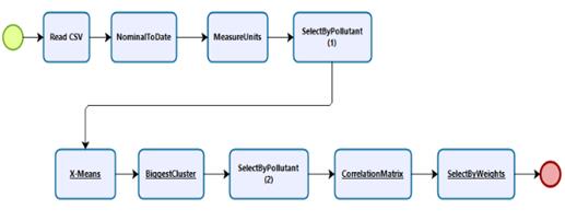
The purpose of the model 1 is threefold: (a) to define the number of data grouping clusters, (b) to obtain all correlations datasets between pollutants, and (c) to identify the incidence between pollutants. To this end, we suggest defining the number of data grouping clusters using X-means algorithm, to structure a correlation matrix using the Pearson or Spearman correlation coefficient depending on data distribution, and define the incidence using "Select by Weights process”. Considering the procedures addressed in the data preparation stage, Figure 2 shows the process to follow in model 1.
The data analysis is focused on the temporality; consequently, the data represented in ReadCSV must be converted to date type. Such conversion is denoted in Nominal2Date. Also, air pollutants measure units must be homogenized. Thus, all pollutants measure units must be converted into the same measurement unit or normalize by Z-Transformation or Range transformation. These conversions are reflected in MeasureUnits. According to the data loggers reflected in Table 1 CO is the only pollutant which needs to be converted.
In order to achieve model 1 first goal, only pollutants columns must be selected in SelectByPollutants(1). Next, the X-means algorithm must be executed. That, it is represented in X-means.
To achieve the second goal in model 1, it is necessary to select the cluster with the greatest number of elements in BiggestCluster. Once again, only pollutants columns are selected in SelectedPollutants(2). Finally, the correlation matrix is developed in CorrelationMatrix. The correlation matrix values reflect the behavior between two pollutants («Quick-R: Correlations», s. f.). There are some factors to consider for its interpretation. First, if the correlation value is less than 0, it indicates that the behavior of a pollutant is inversely proportional to another. This means that the highest values in a pollutant are the lowest values of another pollutant. This is also known as “negative correlation”. Second, if the correlation value is greater than 0, it indicates that the pollutants have a direct correlation. This means that the highest values in a pollutant are highest values in another pollutant. That, it is known as “positive correlation”. Finally, if the correlation value is 0, it indicates that there is no correlation between pollutants. This means that it is not possible to establish senses of covariation.
In order to achieve the third goal of model 1, “Select by Weights process” is applied to the correlation matrix to identify the incidence between the pollutants represented in SelectbyWeights. It is important to consider that a pollutant with an incidence near to 1 may affect another pollutant with a lower value.
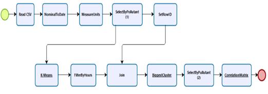
The second model purpose is to obtain the correlations between pollutants in time intervals. We suggest use “Time Rolling Correlations” also denominated “Time Moving Correlations”. In addition, we suggest showing the pollutants behavior using “Simple Moving Average (SMA)” technique to obtain a better data representation. For this, the k value returned by X-means algorithm in model 1 as “k” value is used as priori parameter to structure the clusters using the K-means algorithm. Next, data filter and Time Rolling Correlations techniques are applied to get the correlation matrix. Considering the procedures addressed in the model 1, Figure 3, shows the process to follow in model 2.
In order to apply the K-Means algorithm, only the pollutants columns must be selected represented in SelectedPollutants(1). Once applied K-means represented in K-means, data must be filtered by time intervals. It is represented in FilterByHours. On the other hand, in order to facilitate the data representation by time intervals, an identifier is assigned to the rows corresponding to every pollutants column. That, it is represented in SetRowID. After, in order to recover the hour filed, both SetRowID and FilterByHours are linked in Join. Subsequently, it is necessary to select the cluster with the greater elements number in BiggestCluster. Once more, only pollutants columns are selected in SelectedPollutants(2). Finally, in order to generate the correlation matrix between pollutants “Time Rolling Correlations” is applied. That is represented in CorrelationMatrix. Unlike the correlation matrix in model 1, model 2 presents result in Time Rolling Correlations.
Results stage
Once the models are applied, the knowledge gained needs to be organized and presented in a way that environmental managers or urban planners can use (Wirth, 2000). Statistics plots are useful to reflect the impact of one pollutant on another and help in the identification of the pollutant of major importance.
4. Experimentation
To evaluate the approach proposed in this paper, an experiment using the data collected at the air pollutants monitoring station in Cuenca, Ecuador was conducted. This approach was evaluated by an expert in environmental management, and a statistical expert along with researchers. The aim of the experiment was to evaluate the veracity of the results obtained through this approach and, its utility for environmental management. This section describes in detail the application of the proposed approach, and the results obtained in the context of the city of Cuenca.
Contextualizing the data analysis
Cuenca city is located in the Andean alley of South America at 2500 meters above the sea level. Temperature in Cuenca is 14.7°C on average, which is classified as an oceanic climate (Cfb) in the Köppen and Geige weather map («Clima CUENCA: Temperatura, Climograma y Tabla climática para CUENCA - Climate-Data.org», s. f.). In the experimentation, a real dataset from Cuenca city was used. The air pollutant monitoring station from Cuenca records variables as O3, CO, SO2, NO2 and, PM2.5. Moreover, it reports variables of precipitation; radiation, direction and wind speed; temperature and humidity. Every second, the data is stored in a database registering 864.000 records every day.
Preparing data stage
According to the Data preparation stage detailed in Section III the data for the experimentation was prepared and consisted of an input dataset from a month range random of 215.436 records of 30 days from September 16 to October 15, 2017. The measurements were obtained every minute. The data was corrected through the formula detailed in the data preparation stage in Section III. Also, we seek a clean sample through SQL sentences. Table 2 shows the record number obtained after every step. Once the data preparation was finished, we obtained a dataset with 25.877 records of 17 days from 00:00 am to 24:00 pm. Table 3 shows the initial statistics of this dataset.
Applying the model and results stages
Based in the first model “Data grouping cluster and incidence between pollutants”, for the X-means algorithm was necessary to define the N max of range values to generate the clusters number p from a range 2 ≤ p(min) ≤ p ≤ p(max) ≤ N −1 [21]. To define N, we consulted an expert in air pollution. Thus, the values were defined as N=8 and the result of X-means execution returned p=k=4.
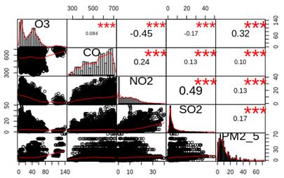
Figure 4, presents the general behavior of all dataset pollutants. On the diagonal, the plot presents the data distribution. In the lower part of the diagonal, the plot presents the data dispersion. At the top of the diagonal, the plot presents the correlation values.
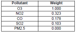
In model 1, we also seek to identify the most relevant pollutant. For that, it is necessary to know the incidence among pollutants. Table 4 shows the incidence among air pollutants.
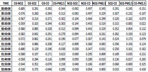
According to Table 4, O3 was the most relevant pollutant in Cuenca city. This means that the O3 pollutant had greater repercussion on other pollutants. No pollutant had an incidence on PM2.5 In model 2, the p-value was used as the K parameter to improve the K-mean efficiency (Kingsy et al., 2016). Once applied the K-means algorithm, we selected the biggest cluster and followed the suggestion of the approach in modelling stage, Section III, we proceeded to analyze the correlation by Time Rolling Correlations. Our aim was to verify the continuous behavior among pollutants throughout the day. Thus, from the original dataset, we analyzed the correlations using Time Rolling Correlations between 60-time series where 1-time series is equivalent to 1 minute and Rolling (moving) it by 10 series. Finally, we show a row per pollutants correlation and time. Table 5, show a summary of the correlation matrix among pollutants at the beginning of a day.
Table 5 shows the behavior with the greatest variation among the correlations. Due to that a value in the correlations is more representative throughout the day; Table 5 reflects more significant data, than data in Figure 4. Moreover, these tables reflect that it is possible to obtain a better performance of K-means in comparison with results in Figure 4.
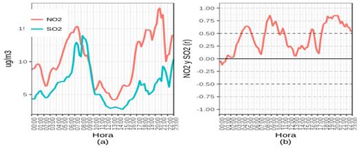
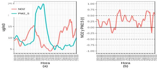
On the other hand, in order to present the knowledge gained in a way that environmental managers or urban planners can use, we generate ten plots created by R software.Figures 5,figura6, figura7 are the most relevant plots. These figures show the pollutants dispersion through smoothed curves throughout the day. These figures are divided into two parts: (a) reflect the pollutants behavior and, (b) reflect the correlation between pollutants. In order to help to compare the correlations values, the first part of the figures (a) shows each pollutant behavior using Simple Moving.
From the results obtained, the evaluators highlighted that the approach returns information close to the reality of Cuenca. The evaluator team consisted in: An Environmental Management Specialist that correlated results generated in this study to the records officially published by the local air monitoring office in their yearly official publications. The Statistics Specialist that assessed and validated the statistical methods used and results obtained. The information returned by the proposed approach was useful to support in the air quality evaluation in Cuenca. Therefore, we claim that the approach can be applied in urban areas with similar characteristics to Cuenca in the Andean region.
5. Conclusions and future work
This paper presents an approach to discovery of knowledge in environmental management. The approach aim is to support environmental managers and urban planners in the decision-making process. The proposed approach allows identifying correlations and the incidence among five harmful air pollutants on the Andean region. Such correlations are analyzed in Time Moving Correlations. The proposed approach is based mainly in X-means and K-means algorithms. We reported a comprehensible experimentation using a real dataset of monitoring station from Cuenca, Ecuador.
In the evaluation, the K-means algorithm reflects a suitable processing time in the grouping task according to the used dataset size. As a mentioned in terms of efficiency (Accuracy and Time Execution) K-means Clustering algorithm presents its self as a good choice, similar results are presented in Doreswamy, Ghoneim, and Manjaunath (2015); Kingsy et al., (2016).
The algorithms and techniques applied were evaluated as positive to extract knowledge from urban areas. This corroborates the hypothesis raised: the application of data mining techniques helps identifying patterns of behavior among several air pollutants. However, additional processes are necessary in order to get complete information which effectively supports the decision making. Therefore, some limitations still need to be overcome. First, the proposed approach does not include other important variables in the air pollution analysis as precipitation or wind speed. Second, the approach does not return information about the causality of incidence. As future work, variables such as precipitation, radiation direction, wind speed, temperature and, the humidity should be included. Also, we will seek to evaluate the approach in other cities in Ecuador.


