Introduction
The degree by which a software product meets user expectations in terms of its ease of use, effectiveness and efficiency, reflects the accomplishment of the intended usability goals of a software development project. Conducting usability testing is central to the realization of such goals because it provides an effective tool to ensure that defects affecting usability are detected before the release of a new product.
In all projects, efficient resource allocation is essential, particularly when the cost of resources is high. Since increasing the amount of user testing sessions directly impacts the project cost, budget constraints will limit the ability to conduct exhaustive user testing. Consequently, from an economical point of view, it is important to ensure that the benefit gained by additional testing is greater than the incurred costs.
Determining the minimum number of participants that exposes most problems in a usability test is a problem that has generated a considerable amount of research and debate during the past two decades. In the early 1990’s, Virzi (1992), Nielsen and Landauer (1993), and Lewis (1994) were the first to publish methods to estimate the size of the smallest sample required to achieve a target proportion of problems discovered in a usability test. Their research, based on empirical data and statistical modelling, allowed them to make three outstanding claims:
Most problems are discovered by the first three to five participants.
The increment in problem discovery after five participants is minimal.
ROI of usability testing can be maximized by minimizing the sample size.
Since their publication, these claims also known as “4±1” or “magic number 5” have generated a great deal of discussion in the usability community, so much so that at the Computer-Human Interaction conference in 2003, a panel was dedicated to discuss this matter (Bevan, et al., 2003).
This paper will focus on, and review the 4±1 model for estimating the sample size required to obtain a proportion of problem discovery of at least 80% in the testing of a web interface. Furthermore, the outcomes of a permutation test will be presented to investigate the effect of small samples on the estimation of the discovery rate.
Background
Three studies were considered for the provision of a suitable base calculation template to estimate sample size: (Virzi, 1992), (Nielsen & Landauer, 1993), and (Lewis, 1994).
Virzi (1992) used empirical data from three experiments and Monte Carlo simulation to conclude that problem discovery rate and the number of participants establish an asymptotic relationship. In his experiments, trained testers observed that the amount of discovered problems depends on the number of participants and the likelihood of discovering a problem. This last parameter is known as problem discovery rate and represents the average of the fraction of problems observed for each user (or the average of the proportion of users that detected each problem). The proportion of problems discovered was modelled with the cumulative binomial probability formula, as follows Formula 1:
Where n is the number of participants, and p is the problem discovery rate.
The problem discovery rate, for a testing session is equal to the quotient between the number of unique problems detected, and the number of problem occurrences observed by all participants.
In (Nielsen & Landauer, 1993) data derived from eleven usability tests, and statistical modelling were used to reach a similar model. In this study, the number of detected problems is estimated as a function of n, p and the total number of problems N, as follows Formula 2:
Both approaches estimate the number of participants (n) required to uncover a goal percentage of problems, with a given problem discovery rate (p), as follows Formula 3.
Lewis (1994) applied the techniques used in (Virzi, 1992) to empirical data from usability testing conducted on a piece of software for office applications. The findings of this study coincided with Virzi’s results. Nevertheless, he noted a potential overestimation of p in small-sample estimation.
Several authors have challenged the soundness of modelling problem rate discovery with a single value for p. Woolrych and Cockton (2001) contend that problems do not affect users uniformly, thus estimation based solely on problem frequency is misleading. Caulton (2001) argues that due to the heterogeneity of users, different types of users will discover different kinds of problems. Therefore, the model should incorporate a term that considers the number of user sub-groups. Turner, Lewis, and Nielsen (2006) responded to criticism of sample size formulae by providing a method to adjust the estimated average problem frequency.
Methodology
The steps involved in this study are summarized as follows:
Obtain data from user testing.
Process data to identify unique and repeated problems.
Calculate parameters and metrics from this data to make observations.
One of the components of the last step in this process is using the calculated parameters to determine the number of user tests or samples required to achieve a level of problem discovery. Later, we employed a permutation test to investigate the distribution of the estimates of the problem discovery rate. In addition, we analyzed the accuracy of the estimation by comparing the mean scores of the estimates against the true value of p. Finally, this number was used to answer the question of whether the number of user tests undertaken was enough to reach a percentage of problem detection greater than 80%.
To review the consistency of the results, the parameters from two different datasets were computed.
Data sources
To obtain data required for the proposed analysis, two datasets were sourced from two independent rounds of testing of a web interface. In the tests, participants were requested to identify usability problems in the interface under study. In total, 34 different respondents participated in both surveys, 17 testers each. The second survey was undertaken two weeks after the first one.
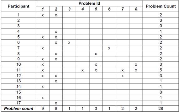
To prepare the user testing data for parameter estimation, two passes were made over each dataset. The first pass was used to identify unique problems, which were catalogued and numbered. Later, the second pass counted which users identified which problem or problems. This process then resulted in a grid structure which shows the problem count for each user test, specifying the problem or problems, observed by each tester. This process also allowed the identification of problems identified by more than one tester. Table 1 shows the processed data from Dataset #2
Parameter estimation
As per Formula 1 the proportion of problems discovered depends on the problem discovery rate (p). To estimate this parameter, the quotient between the number of unique problems and the number of problem occurrences observed by participant is computed. As an example, consider the data in Table 1, in which there are 17 participants, 8 problems, and 28 problem observations (cells containing an “x”), with these values p is 0.21 = 28/(8*17).
Monte Carlo simulation
In many real-life applications, resource constrains prevent to gather enough participants to properly estimate the sample size. In such scenarios, p is estimated from small samples, using rules of thumb such as the “magic number 5”. Hertzum and Jacobsen (2001), and Lewis (2000) investigated the effect of this practice, finding that small-sample estimation produce overestimation of this parameter, which will potentially lead to underestimate the required sample size, and to overestimate the proportion of problems discovered in a usability testing.
To illustrate this, suppose that in Table 1p is computed after the sixth test. The number of problems discovered up until that point is 3, with 7 problem occurrences. The value of p computed with these data would be 0.39 = 7/(3*6), which results in an overestimation of 85% of its true value. If the proportion of problems discovered were projected with the estimated of p, a practitioner would overestimate the number of problems uncovered and stop the testing earlier than needed to achieve a reasonable goal of problem discovery.
Since the selection of the sample to estimate p is arbitrary, different samples (data subsets) will produce different estimates. To investigate the distribution of the estimates, we used Python language and NumPy package to write a program that implements Monte Carlo sampling with 1000 permutations. According with (Lewis, 2000) this number of permutations produce a close approximation to complete factorial combination. The outcomes of the permutation test were used to compute statistics of the distribution of p, and the proportion of problems discovered, as a function of the sample size across permutations.
Note. In the grid a cell containing an “x” denotes the observation of one of the problems by one of the users.
Adjustment of the estimation of p
In (Lewis, 2001) several adjustment techniques are reviewed and synthesized into one method, the author regarded as the most accurate, to adjust the estimate of p. The formula to adjust the value of the p, is Formula 4:
Where n is the sample size used to compute the initial estimate of p, and GT adj is the Good-Turing adjustment to probability space. GT adj is obtained by dividing the number of problems that occurred once by the number of different problems. Going back to the example where p was estimated with a six-participant sample. The estimate for p applying Lewis’ adjustment is 0.229, which compared to true p gives a deviation of 11% (significantly lower than that of the initial estimate).
Results
Parameter estimation
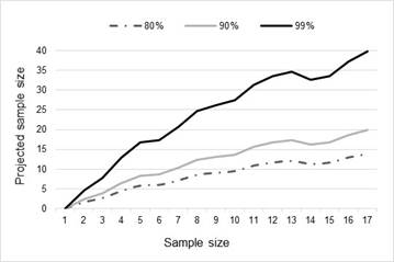
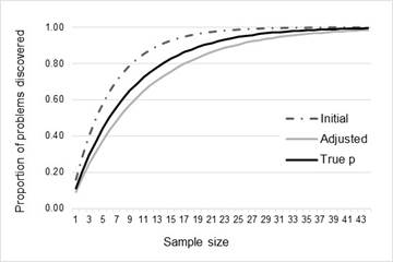
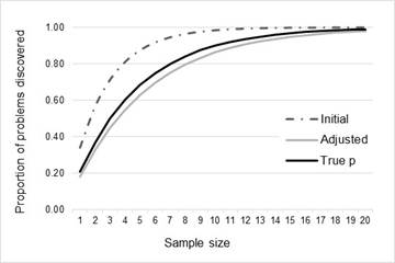
The number of users required to uncover a given percentage of usability problems can be projected as a function of the sample size used to estimate p. Tables Table 2 and Table 3 , and figures Figure 1 and Figure 2 present the estimates of the sample size required to uncover 80%, 90% and 99% of problems computed from datasets 1 and 2.
Statistics of the distributions of the estimation of p
Monte Carlo simulation was undertaken to compute statistics of the distributions of the estimation of p, and the proportion of problems discovered for the two datasets as a function of sample size, across all permutations. The following statistics were computed:
Means of the estimates of p
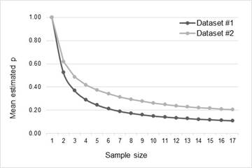
Table 4 and Figure 3 show the distribution of the means of the estimates of p as a function of sample size.
Overestimation ratios of mean estimated p
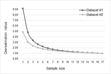
The overestimation ratios were computed against the true value of p of each dataset, and provide a measurement of the deviation of the means of the estimates as a function of sample size. A ratio of 1 indicates no overestimation, while a ratio greater than 1 denotes a overestimation percentage equal to (ratio - 1)*100.
Root medium square error (RMSE) of mean estimated p
The root mean square error is the mean squared difference between each data point and the true value of p for the distribution. Compared to the standard deviation, the RMSE provides a more accurate measure of accuracy because it is sensitive to both the central tendency and variance. The lower the value the RMSE, the lower variance of the measurement. A RMSE of 0 indicates a perfect estimate.
Adjustment of the estimates of mean p
To adjust the estimates of the means of p, the method described in (Lewis, 2001) was used. Table 5 shows statistics of the distribution of adjusted p along with the same statistics of the distribution of the initial estimation Table 7.
Projected proportion of problems and sample for unadjusted, adjusted and true p
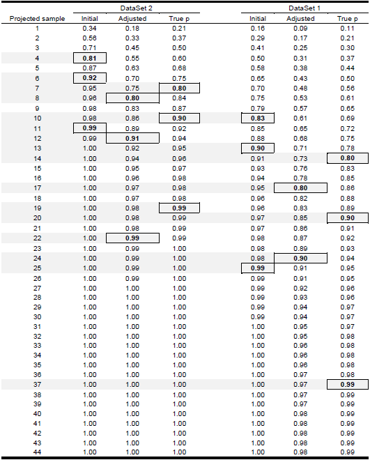
Figure Figure 6, Figure Figure 7 , and Table 8 show the proportion of problems discovered against the projected sample size for the average values of p (initial, adjusted, and true) for both datasets.
Discussion
Parameter estimation
There are two quite significant outcomes from the analysis of the parameter estimation (Figure 1 and Figure 2). The first brings into question the rules of thumb proposed by Virzi (1992), Nielsen and Landauer (1993), and Lewis (1994), in the estimation of the number of user tests required to obtain the desired level of problem discovery.
The second significant outcome is the impact on the sample size of users required for increasing levels of problem discovery. As can be seen from the results from both data-sets, the amount of extra testing required to reach a 99% problem discovery outcome is significantly higher than that of the 90% level. This points towards a higher marginal cost of each extra problem discovered, especially once past the 90% threshold.
The analysis also confirms the commentary by Lewis (1994) on the variability problems associated with using small samples to estimate the number of samples needed for the required level of problem discovery. Even though the goal of Lewis’ adjustments to the p value were to designed improve the calculation of the sample size required for smaller data-sets, the smaller user-test end of the scale for both data-sets showed quite a lot of variability between the test sets, however on both charts the results level out after about eight or nine user tests, thus providing a level of comfort in the suggested sample size results.
This eventual levelling out of results suggests a way to use this type of analysis in practice. If the percentage of problem discovery required is known, after each user test this analysis can be run to determine if more tests are required. For example, if 90% problem discovery is required, if this analysis had been done with Data-Set #1 then it would have been discovered that somewhere between 30 and 40 tests were required, thus pushing the testing past the actual 17 test users. Conversely, testing on Data-Set #2 could have stopped earlier as only 12 or 13 tests were required to hit the 90% problem discovery threshold.
In both scenarios, the question remains as to the “levelling out” point. However, this could be calculated using traditional statistical techniques.
Overestimation and adjustment of p
Analysis of the distribution of the estimates of p confirms the assertion in (Lewis, 2000) that the effect of overestimation is significant for small samples. Figure 3 shows that the means of the estimates increment their deviations exponentially as the size of the sample used to estimate decreases. In Figure 4, all samples less than 8 produce an overestimation greater than 50%, while in Figure 5 the RMS error grows consistently as the sample size shortens. Tables Table 5 and Table 6 confirm this trend. Considering the overestimation ratios, and the RMS errors of the mean estimates, it is evident that the smaller the sample the lower the accuracy of the estimation.
Comparison of the projected proportion of problem detection (and the associated sample size) computed with the initial estimate, the adjusted estimate, and true p (Table 6) shows that the initial estimate reaches a proportion greater than 80% earlier than the adjusted estimated, and the true value of the problem discovery rate. For dataset 1, the projected sample size to achieve 80% of problems is 9 when computed with the initial estimate (5 testers less that the required sample calculated with true p), while the adjusted estimate projects a required sample of 17 users. On the other hand, for dataset 2, the difference between the projected sample computed with the initial estimates and the true sample size is lower (3 users). However, it is worth to note, that the error of estimation increases for 90% and 99% of problem detection. This can be observed in Figure 6 and Figure 7 where the adjusted estimation is closer to the true projection than the initial estimation is.
Several studies (Virzi, 1992), (Nielsen & Landauer, 1993), (Lewis, 1994), (Caulton, 2001), (Turner, Lewis, & Nielsen, 2006), (Hwang & Salvendy , 2010) suggest that when conducting user testing it is sufficient to use rules of thumb such as 4±1and 10±2 to estimate the number of users required.
In our study, we discovered that the use of such rules of thumb would have underestimated the actual number of users required to achieve reasonable levels of problem discovery. In the two data-sets studied, the number of users required to achieve 90% problem discovery were 20 and 10 respectively. This coincides with findings in (Bevan, et al., 2003), (Woolrych & Cockton, 2001), (Spool & Schroeder , 2001), (Faulkner, 2003), and (Lindgaard & Chattratichart , 2007). Furthermore, using small sample sizes can also be problematic as this produces large variability in testing results which cannot be fully adjusted for.
Since the potential costs of achieving problem discovery at the 99% level are significantly higher than that of achieving the 90% level, the use of these levels should be carefully considered unless the development is for applications for which the cost of problems is quite high.
One of the exciting possibilities of the results of this study would be the inclusion of continual problem discovery metrics into a user testing regime. Through continual testing of results, developers could optimize their testing to only include the required number of tests up to the desired problem discovery rate. This has the potential to concentrate testing resources on those cycles that need it rather than equally spreading resources across all cycles.
One possible scenario of use for the 4±1 rule is in time constrained agile cycles, more appropriately towards the start of projects. At this part of the project cycle, there is almost no point in discovering 100% or even 90% of possible problems if development is moving a pace which essentially wipes these problems out or replaces them with new ones.
If a project is severely budget limited, then rules of thumb such as 4±1and 10±2 will also come into play, although we would suggest that the 4±1 rule be only used on relatively simple projects.
This study was conducted in a specific project. However, the applied methodology could be applied to different project task types, different user groups and different environments to see if the rules of thumbs on the number of user tests required can be specified for different type of build projects of differing complexity and task orientation. Such analyses should use at least eight or nine user tests in their parameter estimation to eliminate the small sample size issues that presented in this study.


