Introduction
Nowadays controllers are implemented on digital systems consisting of microprocessors and communication networks. Among some of the alternatives that have efficient resource consumption in a nonperiodic fashion are the self-triggered control techniques (STC), initially proposed by (Velasco, et-al., 2003) - (Anta & Tabuada, 2010), (Mazo, et-al., 2010), (Almeida, et-al., 2011), (Molin & Hirche, 2013). They solve the fundamental problem of determining optimal sampling and efficient processing/communication strategies. Each time the control task is triggered, both the time the next sampling will be performed (sampling rule) and the control action which should be maintained until this event happens, are estimated.
Several approaches aimed at solving the problem of deter- mining optimal sampling rules in STC have been addressed recently. An optimal sampling pattern proposed in (Bini y Buttazzo, 2014) inspired the approach in (Velasco, et-al., 2015), which is analyzed in the present study. This technique describes a sampling rule that generates approximated control actions by solving the continuous-time LQR problem (Astrom & Wittenmark, 1997) at each sample time. The performance guarantee is based on a number of samples over a time interval with a given sampling constraint. The sampling time is calculated by the derivative of a continuous-time LQR problem and the rule produces smaller sampling times while the control action has more variation.
Though the optimal-sampling in (Bini y Buttazzo, 2014) and (Velasco, et-al., 2015) has standard cost lower than the one obtained by periodic sampling techniques, and even than other optimal-sampling approaches i.e. (Gommans, et-al., 2014),(Rosero, et-al., 2017), it has many weaknesses. Since the research is still new there are many open topics, among which two stand out: : (a) clarifying and organizing the implementation on real microprocessor systems, and (b) adapting the approach to cases with disturbances.
To solve problem (a), in (Velasco, et-al., 2015); both a simulated and an experimental set-ups are described. However, a deeper explanation of the paradigm that a designer of control systems should use to put this approach on a microprocessor-based system is not shown.
With regard to problem (b) the approach in (Bini y Buttazzo, 2014); could be restated by inserting robustness to uncertainty in the approach by developing new theory, or on the other hand by using observation techniques. A settlement applying observation in presence of unknown disturbances but on a different STC strategy to that used herein, is presented in (Almeida, et-al., 2012),(Wang & Lemmon, 2010).
To overcome problems (a) and (b), the contribution of this paper is twofold. First, two algorithms are formulated to organize and synthesize the implementation of the approach in (Velasco, et-al., 2015). Second, a time-varying closed-loop observer is applied on the approach in (Velasco, et-al., 2015) in order to make it less sensitive to noise.
The rest of the paper is organized as follows. Section II summarizes the theory on optimal-sampling-inspired self- triggered control (OSISTC). Section III presents the insertion of state observation into the self-triggered control and also the strategies to describe the implementation. Section IV shows the simulations and experiments on a selected plant. At the end, Section V performs the analysis of results and Section VI concludes the article.
Revisiting the optimal-sampling-inspired self-triggered control
This section summarizes the theory on OSISTC extracted from the original works in (Bini y Buttazzo, 2014) and (Velasco, et-al., 2015), and included for better understanding of the subject of study.
Continuous-time dynamics
Consider the linear time-invariant system (LTI) represented in continuous-time by

where  is the state and
  is the continuous control input signal.
  and
and  describe the dynamics of the system, and
  is the weight matrix used to read the state;
  is the initial values of the state.
Sampling
The control input u (k) in (1) is piecewise constant, meaning that it remains with the same value between two consecutive sampling instants, thus
where the control input u
(k)
is updated at discrete times k and the sampling instants are represented by t
k
 . Consecutive sampling instants are separated by sampling intervals
 , and the relationship between instants and intervals is


Continuous-time dynamics
In periodic sampling, a constant sampling interval is considered. The continuous-time dynamics from (1) is discretized using methods taken from (Astrom & Wittenmark, 1997) by

Resulting in the discrete-time LTI system

where the state x (k) is sampled at t k .
The location of the system poles (or eigenvalues of the dynamics matrices A c , A d ) is fundamental to determine/change the stability of the system (Astrom & Wittenmark, 1997). Poles in continuous-time p c become poles in discrete-time p d through
State-feedback control by means of pole placement requires to assign the desired closed-loop poles by hand. Nevertheless, the LQR technique allows to place the poles automatically and optimally. LQR is used by OSISTC at each t
k
considering  as the sampling time.
Linear quadratic regulator
The LQR optimal control problem allows to find an optimal input signal that minimizes the continuous-time and discrete-time infinite-horizon cost functions in (7) and (8) respectively.
Regarding dimensionality in (7) and (8), the weight matrices Q
c
, Q
d
 are positive semi-definite, R
c
, R
d
 are positive definite, and S
c
, S
d
 . Refer to (Arnold & Laub, 1984 to know about the transformation of the weight matrices from their continuous forms Qc, Rc, Sc to their discrete versions Qd, Rd, Sd.
Optimal sampling-inspired self-triggered control
The approach in (Velasco, et-al., 2015) involves designing both a sampling rule as a piecewise control input, such that the LQR cost is minimied.
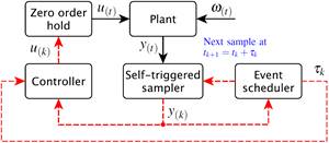
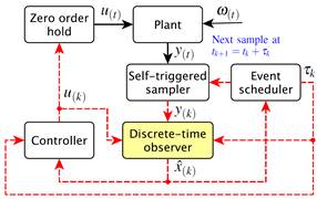
Fig. 1: Original architecture of the self-triggered feedback control. Solid lines denote continuous-time signals and dashed lines denote signals updated only at each sampling time.
Additionally, the periodicity of execution of the controller is relaxed so that consumption of resources is diminishing. Then, the sampling rule is
Where an upper bound on the sampling intervals is given by ; similarly
  modifies the degree of density of the sampling sequence (smaller
  yields denser sampling instants and vice versa). By minimizing the continuous-time cost function (7) an optimal continuous-time feedback gain K
c
is found once. According to (Bini y Buttazzo, 2014) and (Velasco, et-al., 2015) there exist optimal settings for the exponent
  which influences the density of the samples set; with
  the sampling becomes regular (periodic).
Additionally, from (Velasco, et-al., 2015) the piecewise optimal control signal expressed in linear feedback form is:
where  is calculated at each controller execution
  . Its value is obtained by solving the discrete-time LQR problem (8) considering a fixed sampling period
 .
.
On the Implementation of OSISTC
The model of the proposed approach as well as the guide- lines for its implementation are explained in this section. This corresponds to the main contribution of the work.
Original OSISTC architecture
Figure 1 is used to ensure better understanding of the original OSISTC scheme. In this configuration the output of the plant y(t) is sampled by the self-triggered sampler at each  ; the measured state y(k) is used by both the event scheduler and the controller. The event scheduler is responsible for calculating when the next sampling time tk+1 will be executed by means of (9). The controller computes the control action using both (2) and (10). The control input u(k) is kept constant along the entire sampling interval
  in a zero-order hold manner.
In the same Figure 1, the bounded exogenous disturbances  are not treated in any way, causing noisy states and affecting the system performance. With respect to both the event scheduler and the controller, they base their procedures on the measured state y
(k)
(or on the error e
(k)
when there is a reference). Thus, the insertion of noise into the states leads to the emergence of uncertainty in both the linear piece-wise control u
(k)
and the sampling interval
  .
.
Discrete-time observer
An observer constitutes a computer copy of the observers dynamic system (5) whose predicted states  converge to the real states x
(k)
by reducing the observer’s output error
  . The discrete-time Luenberger observer proposed in (Luenberger, 1971) and shown in Fig. 2 is a state estimator which works properly in presence of unknown disturbances; see (Astrom & Wittenmark, 1997) for better understanding. Then, the system in (5) is reformulated as
where  is the state estimate and
  is the output estimate.
  is the observer gain matrix.
In (11), if the pair (A
d
,C) is completely observable, the dual system ( ,
, ,
, ) is completely reachable. Then, an observer gain matrix L
d
for the dual system can be designed and the eigenvalues (poles) of
  can be arbitrarily placed (Luenberger, 1971). Consider that the eigenvalues of a matrix
  are equal to the eigenvalues of its transpose
 .
.
Proposed OSISTC architecture based on observer
Figure 3 shows the proposed self-triggered architecture in which the use of a discrete-time observer stands out to deal with noise ω
(t)
. Assuming that the pair ( , C) is observable along the set of all possible sampling intervals
 , the eigenvalues of
  can be placed arbitrarily (Luenberger, 1971). Notice that the dynamics now depends on
  because
  is a time varying matrix. The discrete poles in (6) are also dependent on the sampling interval
 , as in
In this context the observer needs to solve a new pole placement at each execution, since the discrete dynamics matrices and the discrete poles are dependent on the sampling interval . This implies that the observer has a different gain matrix
  at each execution. Then, considering the changing dynamics, the system in (11) becomes
where  and
and  are discretized matrices for a sampling interval
  , u(k) is the linear piecewise control action calculated by (10), and
  is the gain matrix of the sampling-dependent observer.
Problems considered
There are several drawbacks in assembling both the OSISTC controller and the time-varying observer on a real-time control system.
The first issue has to do with calculation of the controller gain matrix in (10) by solving the problem in (8) through recursive computation of the discrete algebraic Ricatti equation (DARE) until convergence (Astrom & Wittenmark, 1997). The second issue is the pole placement solved by Ackermann’s formula (Ackermann, 1977) in order to obtain the observer gain matrix
 .
.
Both processes are computationally expensive and must be performed at each controller execution. If the execution time of the control task is too close to the minimum sampling interval, undesirable effects such as jitter could appear (Paez, et-al., 2016). Particularly in OSISTC, the worst case scenario comes out when the rate of change of the control action is maximal, causing a highest density in the emergence of samples (minimum ).
).
Set of sampling intervals T
The set of sampling intervals  within a closed interval
  is
is
where  is the sampling granularity defined as the least increase-unit for the sampling intervals. Each element of the set can be addressed in this way
Being s the length of T.
The minimum and maximum sampling times,  and
and , as well as
  are chosen following the conditions detailed in (Velasco, et-al., 2015)
where X is the entire state space taken from the physical constraint of the plant, and  is the sampling granularity of the real-time operating system (RTOS) in which the technique will be implemented.
Strategy to calculate the controller gain matrix

The gain  is calculated by brute force for each h
th
element of the set T in (14) by the discrete-time LQR problem (8). Therefore, we obtain a total of s controller gain matrices
  that have the form
Regrouping the elements of all gain matrices according to their position yields a group that is m · n training sets long, where m and n are the dimensions of inputs and states respectively, then
Each training set in (18) is defined in and used to perform a polynomial curve fitting in order to find the coefficients θ of the d-degree polynomials K
ij
(τ
k
). Therefore, we have a total of
  polynomials each one following the form
where superscript (i j) indicates the belonging of coefficients  to polynomial K
ij
(τ
k
); i-row and j-column show the position of polynomials into the gain matrix. Note the change
of τ k instead of τ h since the former is the current sampling interval calculated online through equation (9) on a real controller. Thus, (17) to (19) become
where
Strategy to calculate the observer gain matrix

It is a process similar to that described in subsection III-F. All possible observer gain matrices  are evaluated offline as functions of sampling interval τ
h
.
The error dynamics of the observer is given by the poles of . A rule of thumb considers to place the observer poles five to ten times farther to the left of s-plane than the dominant pole of the system.
By computing  through (4), assigning statically the continuous-time poles and discretizing them by (6) in order to have the vector
  and finally considering C with remains constant, we obtain a total of s observer gain matrices
  by the poles placement method in (Ackermann, 1977) with the form
Using the same regrouping criterion as in (18) a group ,
,  training sets long, is obtained
Subsequently a total of polynomials are calculated with the form
such as in (19). Finally it is obtained
where
Then, on each execution of the actual controller, after calculating the next sampling interval  via (9), each element of the observer gain matrix is computed through a different polynomial in the matrix
 .
.
Results
An experiment on a real plant is presented in order to illustrate the theory introduced in the previous section.
Plant
The experimental plant with form (1) is the same electronic double integrator circuit as the used in (Velasco, et-al., 2015), so advise with that document for further information. The state space representation is
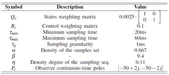
In Table I most important configurations used to design both controller and observer are detailed. These values have been based on recommendations from the literature in (Velasco, et-al., 2015). Note that the poles of the observer have been chosen to be fast enough so that they do not slow down the dynamics of the plant
Controller and observer
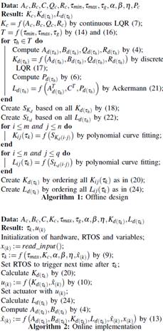
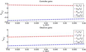
Algorithm 1 has been followed step by step to perform the offline design. In Fig. 4 the gains of both controller and observer evaluated for the set of sampling intervals, are shown by circles. Likewise, fitted curves (continuous lines) roughly describe the behavior of these gains. Additional numerical results are summarized next:
Continuous-time feedback gain
Controller gain matrix which consist of two polynomials, as
Observer gain matrix formed by two polynomials, as in
Implementation on a processor
The development platform comprises the digital signal controller (DSC) dsPIC33FJ256MC710A from Microchip which internally runs the Erika real-time kernel. To learn more about this environment, it is recommended to see the original work in (Lozoya, et-al., 2013); and its references, and the same implementation in (Velasco, et-al., 2015).
The self-triggered controller uses rule (9) to calculate when it will activate itself next time; this value is used to set the RTOS to trigger the next sampling instant. Other functions of the controller are to read the states of the plant x
(k)
through the DSC analog/digital converter, to estimate the states through the observer, and to compute the control action u
(k)
which is applied directly to the plant via pulse width modulation (PWM).
Algorithm 2 has been used to perform the implementation that works on the microcontroller. To calculate the controller gain matrix, two first-degree polynomials that are functions of τ
h
are represented as K
11(τ
h
) and K
12(τ
h
), grouped into  . This is done instead of minimizing DARE. Finally, the observer gain matrix is replaced by a pair of first-degree polynomials L11(τh) and L21(τh), framed within
  . This is done instead of using a pole placement method i.e. Ackermann.
Discussion
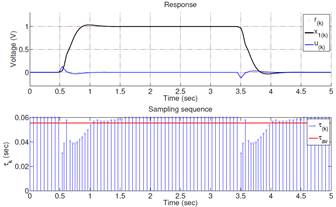
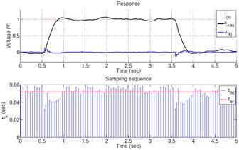
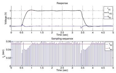
Figures 5 to 7 show the states evolution and the sampling pattern both in simulation and actual implementations when OSISTC is subjected to follow a reference. The establishment times, overshoots, and steady-state errors are almost similar for all cases.
The sampling intervals in the simulation (Fig. 5) lie within the range (31; 60)ms, in the real system without observer (Fig. 6) are within (32; 59)ms, and in the real system with observer (Fig. 7) within (31; 60)ms. The red lines in the sampling sequence graphs correspond to the average sampling, explained later through equation (26).
The observer in Fig. 7 provides noise-free states that stabilize the triggering of sampling periods τk at the same time. The implementation without observer in Fig. 6 tends to shake in steady state since its states have noise, which causes the oscillation of the triggering of sampling periods.
The average sampling metric τav in (Velasco, et-al., 2015); establishes
where N is the number of samples within the experiment/simulation time; larger values of τ av indicate less re- source utilization. In the simulation τ avS = 55.7ms, in the implementation without observer τ avNO = 51.3ms, and in the implementation with observer τ avO = 54.1ms. The average sampling τ avNO is less than τ avO , which means that the implementation with observer has better performance than the implementation presented in (Velasco, et-al., 2015) which has no observer, since it uses less processing resources.
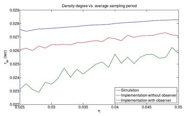
Fig. 8: Comparison of the average sampling period among simulations and implementations with and without observer, with Tmin = 3ms, Tmax = 30ms and n={0.025, 0.026,...,0.050}(Velasco, et-al., 2015);
Figure 8 shows how the sampling average periods behave when the density degree is changed as long as the guarantee in (16) is maintained. The behavior τ avO > τ avNO is recurrent, which allows corroborating the results obtained above.
Conclusions
Some techniques applied at the implementation stage to improve the performance of the method in (Velasco, et-al., 2015) were presented. A polynomial fitted offline to calculate the discrete-time controller gains, was used to replace the online discrete-time LQR problem. A time-varying closed-loop observer has been implemented by polynomial fitting techniques while avoiding the online use of the Ackermann pole placement method.
Simulations and experiments have been confirmed the solution is effective and there could be an open research topic regarding observation techniques in OSISTC. There are interesting performance measures in the literature which could become future work for this study; metrics from (Velasco, et-al., 2015); and (Rosero, et-al., 2017) would allow further evaluation on a real system. A comparison between the implementation with and without observer can be made to determine the true contribution of the latter.


