I. INTRODUCTION

In water resources management and engineering projects, Intensity-Duration-Frequency (IDF) curves are often needed. According to ⁽¹⁾, the IDF curve establishes how the maximum annual average intensity varies in relation to the duration of a specific event. IDF curves are a widely used tool in hydrological design of maximum flows, when rainfall-runoff models such as unit hydrographs or the rational method are used ⁽²⁾. Using this data, a large number of hydrological projects, such as flood discharge designs, bridge construction, and drainage network construction, are defined in relation to the maximum precipitation that could be expected for a given return period ⁽²⁾. The parameters storm duration and intensity of the IDF curve are of great importance in the field of hydrology, as they are the basic elements when it comes to hydrological risk analysis ⁽³⁾. According to ⁽⁴⁾, constructing the IDF relationship of rainfall is one of the main applications of Extreme Value Theory (EVT). IDF relationships are developed based on historical data from time series of rainfall by fitting a theoretical probability distribution to series of annual maximum values ⁽⁵⁾ (that is, maximum values per blocks with a block size of one year) or partial duration series (PDS), also known as peak over threshold series.

In the PDS approach, rainfall events with intensity exceeding the defined high threshold value are considered as the extreme rainfall series and are typically modeled using the Generalized Pareto Distribution (GPD) ⁽⁶⁾. However, ⁽⁷⁾ in Israel analyzed IDF curves based on partial duration series and used both the Generalized Pareto Distribution (GPD) and the Generalized Extreme Value (GEV) distribution, in addition to Gumbel and Log normal distributions, finding that there are not many differences in the results. On the other hand, the extreme rainfall series obtained by extracting the maximum value in each calendar year is generally modeled using the Generalized Extreme Value (GEV) distribution, as seen in works by authors such as ⁽⁸⁾, ⁽⁹⁾, ⁽¹⁰⁾, and ⁽¹¹⁾.

The annual maximum series (AMS) model shows a significant limitation as it does not consider secondary events within a year that may exceed the annual maxima of other years. The PDS overcomes the limitations of AMS by extracting all maximum values that exceed a particular discharge level, called a threshold ⁽¹²⁾. When the threshold is appropriately selected, it can lead to reasonable variability in quantile estimates ⁽¹³⁾, ⁽¹⁴⁾ demonstrated in their research that for records of less than 15 years, the PDS method is superior to the AMS method. On the other hand, ⁽¹⁵⁾ states that PDS is used when the data set is small (< 12 years) or when using return periods less than 5 years. ⁽¹⁶⁾ confirm this information when stating that for modeling return periods less than 10 years (2 and 5 years), PDS tends to produce higher values. This is supported by ⁽¹⁷⁾ in a comparison between PDS and AMS methodologies, demonstrating that for obtaining design storms, PDS is more effective than those imposed by the AMS Methodology since the rainfall exceeds by 4 to 10 %, and therefore is more conservative, and higher results are obtained for return periods between 2 and 5 years.

Despite the advantages shown by the PDS method, the difficulty in determining the appropriate threshold for PDS is a significant obstacle to its widespread use. As expressed by ⁽¹⁸⁾, there is no general recommendation for choosing a suitable threshold.

In their work, ⁽¹⁹⁾ present an equation that shows the relationship between the return period for AMS and PDS, as shown in the following expression (Eq. 1).

Where TP is the return period of the PDS analysis and TA is the return period obtained from AMS. Even for return periods greater than 10 years, this expression can be reduced to TA=TP+1/2, which makes both results, for both PDS and AMS, relatively equal.

On the other hand, another aspect to consider is the variability in data series trends. ⁽²⁰⁾ state that most efforts to develop future IDF curves are limited to individual cities or regions that assume stationarity in precipitation, works by ⁽²¹⁾ and ⁽²²⁾ apply this methodology. Ganguli himself observes that for longer return periods (i.e., 25 years), detectable changes occur in the design storm considering a non-stationary model than the stationary ones. Studies conducted in Malaysia by ⁽²³⁾ demonstrate that for non-stationary models with generalized extreme value functions, there are no clear advantages over similar stationary models.

The selection of the threshold in PDS is the main question that arises, there are several methods for this, but one has not yet been established that applies as a defined law for all cases. ⁽²⁴⁾ estimated a value of peaks per year (λ) ranging from 3 to 15 for homogeneous regions in Italy. Rosbjerg and Madsen (2004) cited in ⁽²⁵⁾ conducted a frequency analysis based on rainfall data using a Bayesian framework in Denmark and suggested a value of λ between 2 and 3. Deidda (2010) cited by ⁽²⁶⁾ developed a multiple threshold method, which is based on parameter estimates within a range of thresholds u>u* and provides a robust fit of the GPD regardless of data resolution or rounding. Regarding the choice of the optimal threshold u*, it should be noted that it should be selected large enough to reliably consider that the distribution of exceedances approaches a GPD, but low enough to keep the estimation variance small. ⁽²⁷⁾ conducted a comparison between PDS and AMS methods, where for obtaining the threshold they choose the minimum value of each duration from the AMS dataset to extract the PDS data. According to ⁽²⁸⁾, since the selection of the threshold is an iterative process, one could easily choose any higher or even lower threshold value, but the lower threshold offers some advantages in terms of sample size. In their study, the author himself states that the results of statistical tests were considerably better if more data points are added. ⁽²⁹⁾ predetermined the threshold values during the selection of rainfall data.

Human errors, such as data entry mistakes, can lead to the presence of outliers or atypical values in the data. Despite the ambiguity in providing a clear definition, an outlier is generally considered to be a data point that significantly differs from other data points or does not fit the expected normal pattern of the phenomenon it represents ⁽³⁰⁾. According to ⁽³¹⁾, they are data points that are extremely distant from the majority of other data points.

There are three types of outliers that a researcher may encounter ⁽¹⁾:

Vertical outliers: These are extreme observations in the dependent variable.

Good leverage points: These are extremes in both dependent and independent variables but fall on or near the regression line.

Bad leverage points: These are outliers in the independent variables.

There is no solid theoretical basis to justify the choice of a specific probability distribution function, nor a theoretical procedure to define a probabilistic model as the best one in a frequency analysis contrasted with different probabilistic models ⁽³²⁾. The author himself established a definitive conclusion, stating that the competence of a probabilistic model in fitting hydrological data is directly related to the flexibility and form of the probability distribution function. Moreover, the more parameters a model contains, the more versatile its probability distribution function will be, adapting to the data.

The formulation proposed by Sherman in (1931), cited by ⁽³³⁾, has universalized the mathematical and graphical representation for calculating intensity (i)-duration (d)-frequency (T) curves worldwide.

In Cuba, ⁽³⁴⁾ conducted a study and proposed a methodology for creating IDF curves in our country. Subsequent research has been conducted, such as that by ⁽³⁵⁾ and ⁽³⁶⁾, both focusing on AMS. In this case, a different methodology is intended to be employed, as there is a small dataset of pluviographic records, specifically 13 years of records. The literature consulted previously affirms that for return periods of less than 15 years, the PDS methodology is superior to AMS. With this, the aim is to establish a new methodology to apply in Cuba for meteorological stations with few years of records.

II. MATERIAL AND METHODS

A. Study Area.

The “La Piedra” Meteorological Station (Code 78308) is located in Manicaragua, a municipality belonging to the province of Villa Clara, Cuba (Figure 1). This municipality is situated at latitude 22°9’0.8’’ N and longitude 79°58’43.2’’ W, nestled in the Escambray Mountains in the southern part of Villa Clara, bordering the provinces of Cienfuegos to the west and Sancti Spíritus to the east. It covers an area of 1066.0 km2, making it the largest municipality in terms of surface area in the province, encompassing the southern portion, resembling a triangle with one of its vertices pointing south, at the intersection point of the provincial boundaries of Villa Clara, Cienfuegos, and Sancti Spíritus. Due to its geographical location, it experiences the influence of a warm humid tropical climate. Precipitation is regulated by the regime of the Northeast Trade Winds, which interact perpendicularly with the moist air masses from higher altitude regions, leading to intense processes with a marked increase in precipitation.

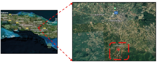
Fig. 1 a) Geographical location of the central region of Cuba, b) Area where the La Piedra Meteorological Station is located. 

An analysis of the pluviographic data recorded during the period 2006-2019 (13 years) was conducted. A study of the maximum precipitation values at the La Piedra Meteorological Station was performed. The results are presented in the form of partial series, considering different time ranges: 20, 40, 60, 90, 120, 150, 240, 300, 720, 1440, 2880, and 4320 minutes.

It is important to mention that there are some limitations due to the lack of records for the year 2018, as the data recording sheets were lost. Additionally, records are occasionally interrupted for short periods due to breakdowns, maintenance, and instrument malfunctions. Another major limitation is the scarcity of recorded years, resulting from the few years the meteorological station has been in operation.

B. Flow Chart.

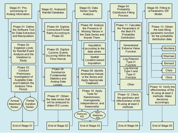
The methodological scheme shown in Figure 2 can be applied to the development of IFD curves in stations that have analog and/or digital data records. It is divided into five stages and 14 phases.

Fig. 2. Methodologicalscheme used in this study. 

Stage 01. The partial duration series of precipitation were collected from the rainfall data recorded at the La Piedra Meteorological Station. Prior to this, the necessary conditions for the analysis of rainy events were established. To process the analog/digital information volumes, Excel, SPSS, and R software were employed.

Stage 02. The database of the selected rainfall parameters to be analyzed was designed with the aim of summarizing the essential components of the IFD analysis in each event, as well as other variables that may be of interest in other research. Since rainfall could be described in various ways as a completely random phenomenon, data were extracted from precipitation hyetographs or mass curves that reflect the statistical behavior of the rainfall shape, as reflected by ⁽³⁶⁾. It was necessary to select a threshold, for which a value was chosen in such a way as to satisfy the condition of independence of the series. A higher threshold value allows us to ensure greater probability of independence, but reduces the number of events in the series, which means a loss of valuable information. On the other hand, a lower threshold value provides a greater number of events in the series, thus allowing for a more reliable parameter estimation, but at the same time increases the possibility of independence. Therefore, a threshold was used that satisfies the condition of independence, while also allowing us to have the largest amount of data possible from the series. The procedure was carried out in such a way that a λ value between 2 and 3 was obtained. An attempt was made to obtain a number of peaks as close to 3 as possible in order to have a larger sample of data considering the limited number of years, as there are only thirteen years of records available.

Stage 03. Demonstrating the quality of the data obtained in the analysis of rainfall events was crucial to ensure the reliability of the predictions. In this regard, the treatment of anomalous data played a fundamental role in avoiding biases in the predictions. The application of sensitivity analysis methods in the analysis of outliers became an essential tool to reduce the uncertainty associated with an IFD curve study. For the analysis of anomalous hydrological data, the US-WRC (United States-Water Resources Council) method was employed. This method is recommended by ⁽³⁷⁾ and ⁽³⁸⁾, where it is cautioned that to apply it, it is necessary to assume that the logarithms or another function of the hydrological series are normally distributed, as the test is only applicable to samples obtained from a normal population. Therefore, to implement the test, Eq.1 and Eq.3 are calculated:

Where, x y s represent the mean and standard of the natural logarithms of the sample, respectively. The KN statistic refers to the Grubbs and Beck table, which is tabulated for different sample sizes and levels of significance, and N denotes the sample size, while XH is the upper limit of the test and XL is the lower limit ⁽³⁷⁾.

If 5≤N≤150, KN can be calculated using Eq. 4 (Stedinger and others, 1993 cited in ⁽³⁷⁾):

For the frequency analysis results to be valid, the dataset must meet the statistical criteria of randomness, independence, homogeneity, and stationarity ⁽³⁷⁾. Table 1 shows the test performed for each statistical criterion.

Table I Year and Area of Construction of the Cells of the Abandoned Sanitary Landfill in the City Of Veracruz 

The analysis of extreme hydrological data frequencies, such as floods, droughts, winds, and maximum daily precipitation, is based on accepting that the maximum annual data in the available sample are independent and come from a stationary random process ⁽⁷⁾. The author himself expresses that due to some factors such as changes in land use and impacts of global warming, hydrological data series exhibit trends, which would indicate that they are not stationary. Therefore, it is necessary to check the existence of seasonality in the data series.

The Mann-Kendall test was developed to identify trends and analyze seasonality in data sets. This test, considered non-parametric, was designed to evaluate the presence of non-linear trends and change points in time series. It is commonly used in detecting trends and spatial variations in data related to climate, hydrology, and agrometeorology, as highlighted by ⁽³⁹⁾.

The null hypothesis of trend, denoted as H0, holds that a sample of data arranged in chronological order is independent of each other and follows the same distribution at all time points. ⁽⁴⁰⁾ defines the statistic S as presented in Eq. 5 and Eq. 6:

Where:

When the sample size (n) is equal to or greater than 40, the statistic S follows an approximately normal distribution. In this case, the mean of that distribution is zero and the variance can be calculated using Eq. 7:

Where t is the size of a given tied group and ∑ is the sum of the set of all tied groups in the data sample. The normalized test statistic K is calculated using the Eq. 8:

The statistic K follows a standard normal distribution, which means it has a specific distribution shape with a mean of 0 and a variance of 1. To find the probability (P) associated with the statistic K in your sample data, you can use the cumulative distribution function of the normal distribution, in the form of Eq. 9:

When analyzing sets of independent data without showing any trend, the value of P should hover around 0.5. In situations where the data exhibit a clear trend towards increasing values, the value of P tends to approach 1. On the other hand, if the trend is marked in a downward direction, the value of P approaches 0. If the sample data are serially correlated, it will be necessary to whiten the data beforehand and apply a correction to calculate the variance ⁽³⁷⁾.

When we are seeking linear trend in a dataset, we commonly use the least squares estimation technique via linear regression to calculate the slope. However, this approach is reliable only if there is no systematic correlation between consecutive observations (serial correlation). Additionally, it is important to note that this method can be heavily influenced by outliers in the data, meaning that an unusual data point can have a significant impact on the slope estimation. Sen (1968) developed a more robust method ⁽³⁶⁾, ⁽³⁷⁾.

The slope of the trend was calculated as Eq. 10:

The trend slope β was estimated using the formula where Q is the resulting value and xi and xj represent the data values at times i and j. If β is positive, it indicates an upward trend, while if it is negative, it signals a downward trend.

The Sen’s slope estimator is simply the median of the N’ values of β. This approach is applied in the same way, whether we have one or multiple observations per time period.

Sen (1968) proposed a non-parametric method to calculate a confidence interval for the slope. However, in practice, a simpler method based on the normal approximation is more commonly used. To calculate this, we require the standard deviation of the Mann-Kendall statistic, S ⁽³⁷⁾. In simpler terms, we need to know how much the Mann-Kendall statistic S varies in order to perform calculations related to its distribution and statistical significance.

Stage 04. Identifying the probability function best fitting the data for the evaluated conditions and the proposed significance level was essential. Fit was assessed using analytical and probabilistic methods to ensure the correct choice of the distribution function and the results of its parameters.

In the field of hydrology, probability distributions are essential tools used to analyze precipitation amounts and patterns in time series. To describe rainfall events, three distributions were employed: ⁽¹⁾ Generalized Extreme Value (GEV), ⁽²⁾ Generalized Pareto ⁽²⁹⁾, ⁽³⁾ Johnson SB. Eq.11, Eq.12, and Eq.13 show the probability density function of GEV, the Generalized Pareto distribution, and the probability density function (Johnson, 1949), ⁽³⁴⁾, respectively:

Where μ is the location parameter, σ is the scale parameter, and ξ is the shape parameter. When ξ=0, the GEV reduces to the type I extreme value distribution (Gumbel). When ξ>0, the tail of the distribution is heavier, and when ξ<0, the tail is lighter.

Where κ is a shape parameter, ξ is the location parameter, and α is the scale parameter.

ε, λ: Location and scale parameters.

γ, δ: Shape parameters representing skewness and kurtosis, respectively.

Parameter estimation A very tempting method from a statistical point of view is the maximum likelihood method. It consists of selecting the parameters that give a fitting distribution the greatest statistical coherence possible with the observed sample.

The method of maximum likelihood is the most commonly used method to find the parameter values that make the observed data most probable under the proposed model, as affirmed by Millar (2011) and Pawitan (2001), both cited by ⁽²⁴⁾. The author himself expresses that the method provides biased estimates, hence researchers strive to develop nearly unbiased estimators for the parameters of various distributions.

Goodness of fit ⁽³⁰⁾ stated that many of the problems observed in numerous research studies stem from the incorrect use of test statistics, which occurs when they are applied inappropriately. This can be due to various factors:

Lack of knowledge of both descriptive and inferential statistics.

Limited understanding of research methodology.

Shortage of research-oriented faculty members.

Inadequate familiarity with statistical software.

These four aspects directly influence the conduct of research. If any of them is not understood or applied properly, the research would exhibit significant deficiencies. ⁽³⁷⁾ explains that in hydrology, there are various rigorous and effective statistical tests to evaluate whether it is plausible to conclude that a specific set of observations comes from a particular distribution. These tests are called Goodness of Fit Tests. The Kolmogorov-Smirnov test allows for obtaining bounds for each of the observations on a probability plot when the sample has been effectively drawn from the assumed distribution.

This procedure is a non-parametric test that allows testing whether two samples come from the same probabilistic model. Suppose we have two samples of total size N=m+n composed of observations x1, x2, x3, …, xn e y1, y2, y3,…, ym. The test assumes that the variables x e y are mutually independent and that each x comes from the same continuous population P1 and each y comes from another continuous population P2. The null hypothesis is that both distributions are identical, meaning they are two samples from the same population ⁽³⁶⁾.

The Kolmogorov-Smirnov test was used due to its ability to reasonably assume that observations could follow the specific distribution in question. It is straightforward to calculate and apply, and it does not require data grouping, unlike the Chi-square test. Additionally, it has the advantage of being applicable to samples of any size, unlike the Chi-square test, which requires a minimum sample size.

Stage 05. The results of the probability function were parameterized into mathematical models of the form f(I)=(D) for different T, or f(I)=(D; T), in order to verify the effectiveness of the fits. If necessary, a point of inflection in the data series was identified, contributing to obtaining more precise results with less margin of error. Models for Intensity-Frequency-Duration curves: In this study, we focused on fitting the models proposed by Montana, Sherman, Bernard, and Chow according to ⁽³³⁾, ⁽³⁶⁾, equations 14, 15, 16and 17.

Where: 𝑖 𝑑 𝑇 It represents the maximum precipitation intensity, measured in mm/min or mm/h. T is the return period in years, d is the duration of precipitation in minutes, and k, m, θ and n are the parameters that must be estimated to fit the curve.

III. RESULTS AND DISCUSSION

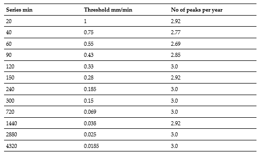
The Table II shows the selection of thresholds is shown below, indicating the threshold and the number of resulting peaks in each of the time series.

Table II RESULTS OF THRESHOLD SELECTION AND NUMBER OF PEAKS FOR EACH SERIES 

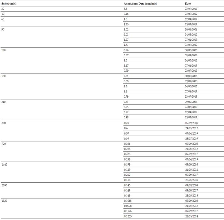
The data processing was done with the assistance of the R software. The US-WRC method was applied, which extracts the outlier data from each series. Table III displays these outlier data.

Table II RESULTS OF THRESHOLD SELECTION AND NUMBER OF PEAKS FOR EACH SERIES 

The data shown in Table III were removed from the series for exceeding 10 % above the upper limits of the US-WRC model for a 95 % confidence level.

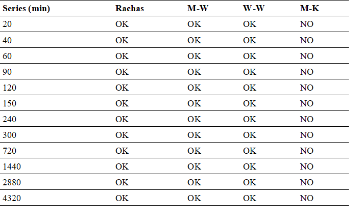
The results of the quality tests conducted on the partial duration series as recommended by the ⁽³⁶⁾ included Runs, Mann-Whitney (M-W), Wald-Wolfowitz (W-W), and Mann-Kendall (M-K) tests and are summarized in Table IV. The expression ‘OK’ means that the null hypothesis is accepted, and the word ‘NO’ means that the null hypothesis is not accepted, indicating that:

The series is random at a significance level of 5 % (Runs Test).

The series is independent at a significance level of 5 % (Wald-Wolfowitz Test).

The series is homogeneous at a significance level of 5 % (Mann-Whitney Test).

The series is seasonal at a significance level of 5 % (Mann-Kendall Test).

Table IV RESULTS OF QUALITY TESTS FOR EACH DATA SERIES 

According to the results obtained in the quality tests, it has been demonstrated that the data series collected for the La Piedra Meteorological Station are suitable for use in the development of Intensity-Duration-Frequency (IDF) curves. These results highlight the data’s capability to be used in probabilistic analyses, suggesting the suitability of applying non-stationary models in the processing and interpretation of such information, in order to understand and predict climate patterns with greater accuracy and relevance.

Figure 3 shows the results of the analysis using the Generalized Pareto distribution, which has been adjusted using the nearest neighbor method. The results are presented for intervals of 1h, 2h, 4h, and 12h. The adjustment corresponding to the previously mentioned durations is illustrated using the cumulative probability function graph.

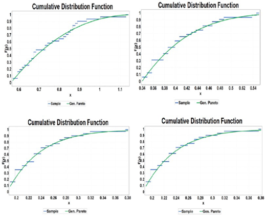
Fig. 3 Fit to the Generalized Pareto cumulative probability function for intervals of a) 1h, b) 2h, c) 4h, d) 12h. 

In Table V, the results of the position and scale parameters derived from this analysis are detailed.

Table V PARAMETERS OF THE GENERALIZED PARETO PROBABILITY DISTRIBUTION OBTAINED FOR THE 1H, 2H, 4H, 12H SERIES 

The Kolmogorov-Smirnov goodness-of-fit test is conducted to assess the suitability of the ⁽¹⁾ Generalized Pareto, ⁽²⁾ Generalized Extreme Value (ξ=0), ⁽³⁾ Johnson SB functions in obtaining the optimal probability function. With a significance level of 95 %, the test results indicate that the fit by the Generalized Pareto is statistically more effective.

The application of the Montana, Sherman, Bernard, and Chow models to fit the results of the Pareto probability function in a partial duration series did not yield favorable results. In this context, we rely on the Pearson correlation coefficient, detailed in Table VI, along with the values of k, m, θ, C, and n associated with each model.

Table VI PARAMETERS OBTAINED AND PEARSON CORRELATION RESULTS FOR THE APPLIED MODELS 

As a result, the suggestion is to divide the series into two segments: the first covering up to 12 hours and the second beyond 12 hours. By implementing this modification in the models, Table VII presents new values for k, m, θ, C, and n, along with a new Pearson correlation coefficient.

Table VII PARAMETERS OBTAINED AND PEARSON CORRELATION RESULTS FOR THE APPLIED MODELS WITH DURATIONS LESS THAN AND GREATER THAN 12 HOURS 

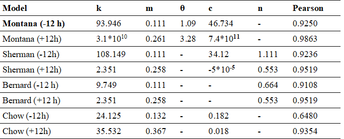
According to the data presented in Table VII, it is concluded that the Montana model proves to be the most suitable for fitting the results of the Generalized Pareto probability distribution. This analysis supports the choice of the Montana model as the one that best fits the data of the series in question, and Equation 18 represents the conclusive formula used for the analysis at the corresponding station.

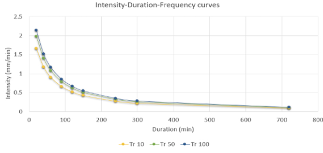
In Figure 4, the graphical representation of the Montana fitting function specifically for the La Piedra Meteorological Station is visually presented.

Fig. 4 Graph of Intensity-Duration-Frequency (IDF) curves for the La Piedra Meteorological Station. 

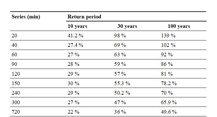
Table VIII shows the numerical percentage difference between the values obtained using the Montana method and the values from NC 1239-2018. For this purpose, the results of the Montana method were compared with those of NC 1239-2018, calculating the difference between both sets of data.

Table VIII COMPARISON BETWEEN THE RESULTS OBTAINED BY THE MONTANA METHOD AND NC 1239-2018 

The difference was expressed as a percentage to clearly identify the maximum deviation between the compared values. It was determined that the greatest discrepancy, 139 %, was observed for a return period of 100 years and a rainfall duration of 20 minutes.

IV. CONCLUSION

After conducting the study and analysis of the data obtained throughout this research, the following conclusions are drawn:

The collected data cover a period of 13 years of pluviographic records from the La Piedra Meteorological Station. During the processing of this data, series representing partial duration for intervals of 20, 40, 60, 90, 120, 150, 240, 300, 720, 1440, 2880, and 4320 minutes were generated.

Pluviographic records for the year 2018 were not available due to total loss.

41 values considered outliers were identified using the US-WRC method. These values were excluded from our analysis due to the lack of information about their origin or source.

The data series underwent analysis to verify their randomness, independence, homogeneity, and seasonality. As a result of this analysis, the hypotheses were corroborated, and it was concluded that a non-stationary IDF model would accurately represent the studied phenomenon.

The Pareto distribution was applied to the data series, and it was verified, through the Kolmogorov-Smirnov method, that this distribution fits the data adequately. This fit was highlighted when compared to the Johnson SB and Generalized Extreme Value distributions, with the Pareto distribution yielding the most favorable results in comparison.

The Montana model achieved parameterization with a more significant correlation when applied to data from the probability distribution. It is important to note that this was achieved by dividing the series into two categories: durations less than 720 minutes and durations greater than this figure. This division led to the formulation of a Montana model with two equations presenting different parameters.

The results of this research present data developed through the Montana method, which, when compared with NC 1239-2018, showed a difference in values exceeding 100 %.