I. INTRODUCTION

Variable temperature is considered a fundamental climatic element. It influences ecosystem function in terrestrial life ^1,2,3. Missing information, data errors, and outliers are problems encountered in the analysis and prediction of climatological phenomena. The difficulties described below are based on environmental, technical, and operational factors that affect the instruments and sensors. Several studies have used mathematical and statistical methods to estimate a fit function to complete missing values based on information from the closest stations ^4,5.

Objective analysis (OA) was used to determine the analytic function that represented the distribution of the data. By observing numerical data at irregularly spaced points, the spatial distribution structure can be reconstructed in two or three dimensions ^5,6,7. This process has been applied for several purposes, including interpolation, data error correction, and smoothing. In most applications, it is incorporated to ensure internal consistency ⁶. It must be emphasized that this methodology has performed spatial and temporal interpolation on the continuous representation of data for weather forecasting, mapping, assimilation analysis, and visualization of climate variables ^8,9

Cressman is considered an interpolation method used to estimate values in a given region; it is based on the contribution of the closest values to an unknown point, which means that estimated values have less influence from more distant points. This approach is known as the nearest neighbor method ^6,10. On the other hand, Barnes is used to interpolate data in a scalar field; it is based on a mesh of cells and a weighting function used to weight the known data near the missing point, resulting in a smooth and accurate procedure that considers the spatial variation of the data ^11,12.

Although these methods are used for spatial interpolation, minimal parameter restrictions are applied for temporal interpolation; because the atmospheric variable distribution can be represented by the sum of an infinite number of independent waves, which is a Fourier integral representation. These findings support the relationship between the weight function and the definition of influenced radio using successive correction techniques. In this way, the estimation of missing data is performed using information from the same station and adjusting the model to the time series ¹³.

The purpose of this investigation was to obtain a smoothed function using the Cressman and Interactive Barnes Objective Map Analysis Scheme as a temporal behavior approximation for the temperature series. Missing data is essential for ensuring the integrity and reliability of the results.

II. MATERIALS AND METHODS

Meteorological stations have reported climatic variables such as temperature (°C), humidity (%), solar radiation (watts/m2), atmospheric pressure (hPa), wind speed (m/s), and wind direction (°), since 2013. This information was recorded in a database as part of the repository in ESPOCH (http://ceaa.espoch.edu.ec:8080/redestaciones/). The Alao station is located at 773499E and 9793173N in Pungalá, Chimborazo (Figure 1). Its altitude is 3064 m a.s.l. It has a territorial extension of approximately 28.133,06 hectares. The hourly mean temperature data contained 8760 observations, corresponding to 2021. These methods were developed using the Jupiter interface in Python, which is an open-source multi- paradigm programming language.

The implementation code is available at: https:// github. com/geaaespoch/Cressman-and- Barnes-method. The weighted mean value was determined by estimating variables. As the sum of the weighted values depends on the distance from the model mesh node to the observation point, the closest values have a greater influence ¹⁴.

Figure. 1 Geographic Position of Alao Station 

Interactive Barnes Objective Map Analysis Scheme (IBOMAS)

The Barnes method (1964) assumes that the two-dimensional distribution of an atmospheric variable is represented by the superposition of harmonic waves, that is, a Fourier integral representation. A weight function is obtained using the separation of variables method for the wave equation. In this context, the probability distribution function of the data was represented by this function.

The Barnes Objective Map analysis has modified the initial Barnes scheme; it considers two weight functions as shown in equation (1) and ^14-16:

()1

And:

()2

Where rm is the distance between the grid point i and observations f(xi), and 0 < λ < 1 is the horizontal wavelength. Furthermore, K and K0 are the parameters of the response function that can be defined by the variance of the data.

The current correction is expressed as the sum of the weighted averages of M observations:

()3

Where the first addend is represented by the Barnes successive correction, and the difference between f(xm)-g0(xm) indicates the adjustment of the interpolation obtained with Barnes weighting to the observed data. In turn, g0(x), a weighted Gaussian function, acts as the initial approximation for performing Barnes interpolation ^{(17, 18)}. Moreover, the function g0(xm) can be interpolated using different interpolation methods ¹⁹.

Unlike the Barnes method, IBOMAS controls the scale of the influence of the surrounding data by adjusting the wavelength, thus allowing the interpolation to be customized according to specific needs. Additionally, the convergence of the correction is achieved after at least two passes.

Cressman method

Cressman's method (1959) is used to estimate values at unsampled points within a region. This method is based on the idea that values near an unknown point have a greater influence on the estimated values than those further away. Cressman's method is similar to a nearest- neighbor interpolation technique and is used in geophysical and environmental applications. ^5,6,14

In our case, it used the weighted average of the observed values to calculate the estimated value at an unknown location, where the weights were determined by the Euclidean distance.

Mathematically, it can be expressed as

()4

Where fi represents the observed data. In this case, Cressman's method was used, with one iteration defined by the radius of influence for the unsampled point and a weighting function that depends on its distance to the unsampled point and the radius of influence.

()5

And

()6

Where di is the Euclidean distance between the sampled and unsampled points, and R is the radius of influence value.

Evaluation of the performance of the missing data estimation methods

To validate these methods, calculating the error and precision metrics is essential to evaluate the performance and compare the models, thus selecting the best fit. Therefore, the mean square error (MSE), mean absolute error (MAE), mean square error (MSE), residual sum of squares (RSS), coefficient of determination (R²) and accuracy allowed to measure the differences between the observed and estimated values. It is an objective tool for measuring the performance of a model and improving its precision and accuracy (20).

()7

()8

()9

()10

()11

Where M represents the total amount of data, zi refers to the observed temperature in a specific element i, represent the estimated temperature, indicates the average of the estimated data, and refers to the average data observed ²⁰.

III. RESULTS

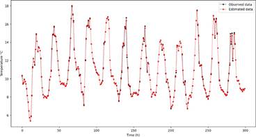
The analysis of the Alao Meteorological Station database reported 8760 observations in 2021, with 20% missing data. The Cressman and Barnes methods were used to fill in missing data for time temperature variable series reports. The Cressman method estimates the missing values of the study variable, with radii values of 10, 30, and 60, using the weighted mean function and Euclidean metric (Figure. 2).

Figure 2 illustrates the comparison between the original and estimated data using Cressman's method. The original data, represented by the solid blue line, are plotted against the estimated data, depicted by the dashed red line. The x-axis represents the time, ranging from 0 to 300, whereas the y-axis represents the measured values, ranging from 0 to 18. The estimated data closely followed the original data, indicating a high level of accuracy in interpolation. The overall pattern and peaks of the estimated data aligned well with those of the original data, although minor deviations were observed at certain points. Despite these small discrepancies, the general trends and fluctuations were accurately captured. To quantify the accuracy, statistical metrics such as the Mean Absolute Error (MAE), Root Mean Squared Error (RMSE), and correlation coefficient were calculated between the original and estimated data. These observations suggest that Cressman's method effectively estimates missing or unsampled data points within a region while maintaining a high level of fidelity to the original dataset.

Figure. 2 Cressman method. 

IBOMAS uses a Gaussian weighted function such that not all observations are removed in the first pass, allowing estimates to be obtained at all points, as shown in Figure 3. The estimated data presented variations and trends that were similar to those of the observed data. Similarly, IBOMAS in the second pass exhibited greater convergence between the data, as shown in Figures 3-4.

Figure. 3 First pass - IBOMAS 

The analysis presented in Figure 3 demonstrates the effectiveness of the IBOMAS in estimating the original dataset. The graph compares the original data (depicted by the solid blue lines) with the estimated data (depicted by the red dashed lines) across 300 data points. The y-axis values range from approximately 4 to 18, indicating variability in the dataset. The estimated data closely followed the trend of the original data, thereby capturing periodic patterns with high accuracy. Although minor discrepancies were observed, particularly at the peaks and troughs, these deviations were minimal and did not significantly affect overall accuracy. The results confirm that the IBOMAS method provides a reliable and precise estimation of the original data, effectively capturing the underlying patterns and periodic behavior present in the dataset.

Figure. 4 Second pass - IBOMAS. 

The analysis depicted in Figure 4 highlights the performance of the IBOMAS in estimating the original dataset. The graph illustrates the original data (solid blue lines) compared with the estimated data (red dashed lines) over a span of 300 data points. The y-axis values, ranging from approximately fourth to eighteen, display the variability of the dataset. The estimated data successfully mirrored the trend of the original data and accurately captured periodic patterns. Although minor discrepancies were noticeable, particularly at the peaks and troughs, these deviations were minimal and did not significantly compromise overall accuracy. These results confirm that IBOMAS is highly effective in estimating the original data and accurately capturing the inherent patterns and periodic behaviors within the dataset.

In the context of the Cressman method, the choice of influence radius was influenced by the temporal scale, with a delta t of 48 h. Hence, it is sensible to employ the influence radii of 10, 30, and 60. The results indicate that an optimal fit was achieved with a radius of ten for both the Cressman and IBOMAS methods. However, with Cressman, discrepancies emerged with radii of 30 and 60, leading to underestimation and overestimation of the data, respectively, as shown in Figs. 6 and 7. Conversely, IBOMAS converges with the observed data across a range of influence radii, as illustrated in Figs. 5-7.

Figure. 5 Estimation Methods R=10 

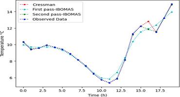
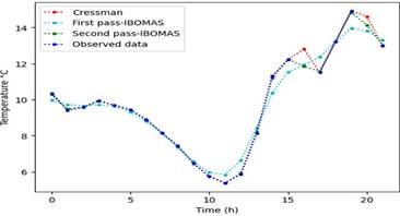
Figure 5 compares different estimation methods for temperature over a 24-hour period, highlighting the performance of Cressman's method, the first pass of the IBOMAS method, and the second pass of the IBOMAS method against the original data. Each method followed the general trend of the original data, which showed a temperature range (6 - 14°C). However, the IBOMAS method (both first and second passes) demonstrated a closer alignment with the original data points, indicating a higher accuracy compared to Cressman’s method. Notably, all methods capture a significant drop in temperature around the 10-hour mark and a sharp rise around 15-17 hours. The IBOMAS method, particularly the second pass, showed superior precision, making it more reliable than Cressman´s method for accurate temperature estimation.

Figure. 6 Estimation Methods R=30 

Figure 6 illustrates the comparison of temperature estimation methods over a 24-hour period with a radius parameter R=30. This is in contrast with Cressman's method, the first pass of IBOMAS, and the second pass of IBOMAS using the original data. All the methods generally followed the trend of the original temperature data, which fluctuated between approximately 6°C and 14°C. However, the IBOMAS method, particularly the second pass, aligns more closely with the original data points, demonstrating higher accuracy. The graph highlights the key points where all methods show a significant drop in temperature around the 10-hour mark and a sharp rise between 15 and 17h. Despite the overall trend, Cressman’s method showed less precision than both the IBOMAS passes. This analysis indicates that, for more accurate temperature estimations, the second pass of IBOMAS is the most reliable, followed by the first pass, with Cressman's method having the least accuracy.

Figure 7 presents a comparison of the temperature estimation methods over a 24-hour period with a radius parameter R = 60. It evaluates the performance of Cressman's method, the first pass of IBOMAS, and the second pass of IBOMAS against the original temperature data. All methods tracked the trend of the original data, which ranged from approximately 6°C to 14°C. IBOMAS, particularly the second pass, exhibited a closer fit to the original data points, indicating superior accuracy. Key observations include a significant temperature drop around the 10-hour mark and a sharp increase between 15 and 17 h.

Figure. 7 Estimation Methods R=60 

Although all methods capture these trends, Cressman's method shows less precision than both IBOMAS passes. This analysis suggests that, for a more accurate temperature estimation, the second pass of IBOMAS is the most reliable, followed by the first pass, with Cressman's method being the least precise.

Figure 5. It is visualized that the IBOMAS first and second pass model fit the observed data, while little divergence is observed in Cressman concerning radii 30 and 60. The ability of the models to fit the observed data supports their effectiveness in filling the missing values.

Error analysis

In meteorology and climatology, the utilization of interpolation methods is of paramount importance to accurately represent atmospheric phenomena. A comparison of different interpolation techniques, such as Cressman and IBOMAS, is significant because it provides insights into their efficacy in handling sparse meteorological data. This comparative analysis sheds light on their respective strengths and weaknesses, aiding the refinement of atmospheric modeling techniques. By assessing how each method addresses data sparsity, researchers can gain a deeper understanding of its performance in capturing the atmospheric dynamics. Hence, investigating the error between Cressman and IBOMAS will facilitate advancements in atmospheric science by enhancing the accuracy and reliability of numerical weather prediction models.

Table 1 Error analyses 

The model validation metrics (MAE, MSE, RMSE, R², and accuracy) tended to be close to zero or unity, indicating a good fit to the observed data and greater accuracy and effectiveness of the methods, as shown in Table 1.

The results of this study indicate that the IBOMAS method, particularly in its second pass, demonstrates significantly superior performance in terms of accuracy and explanatory capacity compared with the Cressman method. The choice of the influence radius is a determining factor for the effectiveness of both methods. In the second pass of IBOMAS, a mean squared error of 0.129 was obtained across all evaluated radii, revealing a 22% difference between the passes of IBOMAS in contrast to the 21% variation observed in the Cressman method. Accuracy was assessed using the coefficient of determination, achieving 98% effectiveness in the first pass of IBOMAS and 99.9% in the second, whereas the Cressman method attained 92% effectiveness with an influence radius of 10. These findings suggest that minimizing both the underestimation and overestimation of values can reduce errors and yield more reliable results, thereby recommending the use of IBOMAS to improve missing data estimates in similar geographical contexts.

IV. DISCUSSION

The methodologies of IBOMAS and Cressman employ a half-weight approach, with the distinction that the Cressman weight function is determined based on the distance between the observed values and the influence radius, which is determined subjectively to ensure that all grid points represent the data points as well as possible and are sometimes chosen to limit the effect of a station ²¹. In contrast, IBOMAS utilizes a Gaussian function that uses a scale parameter to compute the weights for neighboring data points based on their distances. Subsequently, the scale parameter is refined by assessing the difference between the estimated data in the first pass and the corresponding observed values, thereby improving accuracy ⁵.

The influence radius is a critical parameter in interpolation because its accuracy is largely dependent on the underlying data distribution. A reduced influence radius (R) may omit the essential information during the interpolation process, leading to excessively smooth and inaccurate estimates. Conversely, an overly broad influence radius can result in the inclusion of irrelevant data, potentially introducing a bias into the results. Therefore, three different influence radii were evaluated: 10 km, 30 km, and 60 km, considering that meteorological stations record data for meteorological variables within a radius of 25 km. It was observed that, in contrast to IBOMAS, the Cressman method was particularly sensitive to the selection of these three influence radii ^{(17, 22, 23)}.

The inherent nature of Cressman poses challenges when the data distribution is uneven. By contrast, IBOMAS ensures that the weights are never nullified by utilizing all observations when estimating the values. Moreover, IBOMAS allows for estimates at all observed points, thereby avoiding artificial discontinuities present in the Cressman method ^2,4,11.

During the first pass, IBOMAS interpolates by employing a scale parameter to calculate the weights for neighboring data points based on their distances. In the second pass, IBOMAS adjusts the scale parameter using the disparity between the imputed data from the first pass and the observed data, thereby enhancing precision. The objective is to reduce the interpolation error with successive passes ²⁴, thereby achieving improved results in which the estimated values closely align with or match the observed data, ultimately attaining acceptable convergence, as shown in Figure 5.

In both the Cressman and IBOMAS methods, the second pass mirrors the observed data. Furthermore, cross-validation methods indicated an accuracy and regression coefficients ranging between 80 and 99.9%. In this study, we conducted evaluations by using various radii. No significant differences were observed for IBOMAS at ratios of 10, 30, and 60. Conversely, in the Cressman method, there was an 11% disparity in the similarity of the estimated data, owing to the dependence of the weighted function on the radius of influence ¹⁴.

Other variations in successive corrections can be evaluated, as indicated in ²⁵, considering the detrended data. The choice of the number of iterations was decided after the analysis, ensuring that the method adequately fits the observed phenomenon.

V. CONCLUSIONS

The analysis of temperature data from the Alao Meteorological Station showed the effectiveness of the Cressman and IBOMAS methods in estimating the missing values. IBOMAS in the second pass showed superior accuracy and better convergence with the original data. This method uses Gaussian weighted functions and multiple iterations to capture periodic patterns and underlying trends with high fidelity.

The Cressman method was effective, although it exhibited limitations with larger radii of influence, resulting in both underestimation and overestimation. A radius of 10 provided the best fit for both methods; however, IBOMAS maintained a better consistency at radii of 30 and 60. In the error analysis, IBOMAS achieved an MAE of 0.129, MSE of 0.103, and R² of 0.991 in its second pass, significantly outperforming Cressman's method. Future studies should consider the implementation of IBOMAS in other geographic contexts, particularly in regions with similar climatic and topographic characteristics, where data distribution may present challenges. Additionally, further research could explore the integration of IBOMAS with machine-learning techniques to enhance the accuracy of the interpolated values