A. Test vehicle

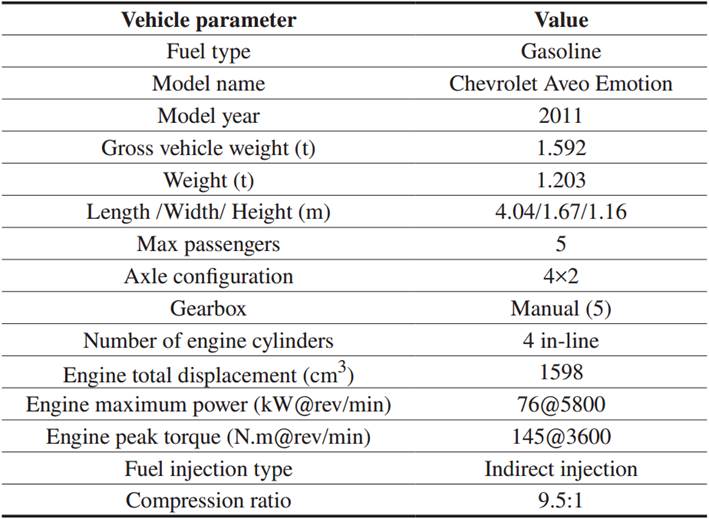
A representative passenger vehicle powered by gasoline of the ecuadorian vehicle fleet was selected to analyze the performance of an engine in real traffic conditions. In fact, in the last decade, this vehicle has been one of the most used models for the taxi service in several cities of Ecuador⁽¹⁷⁾. The tested vehicle was a Chevrolet Aveo Emotion, equipped with an engine of 1.6 liters. In general, the characteristics of the test vehicle are representative of passenger capacity, weight, engine torque and power and gearbox type for the automotive segment of the country.Table Iprovides additional information of the tested vehicle. Moreover, it is important to note that the tested vehicle underwent an exhaustive preventive and corrective maintenance program to guarantee the results of this study. In fact, this maintenance ensured that the vehicle successfully passed the mandatory annual technical inspection required by ecuadorian regulations. Consequently, the evaluated vehicle was in optimal technical condition before the execution of the experimental campaign.

Table I Technical specifications of the tested vehicle 

B. Test route

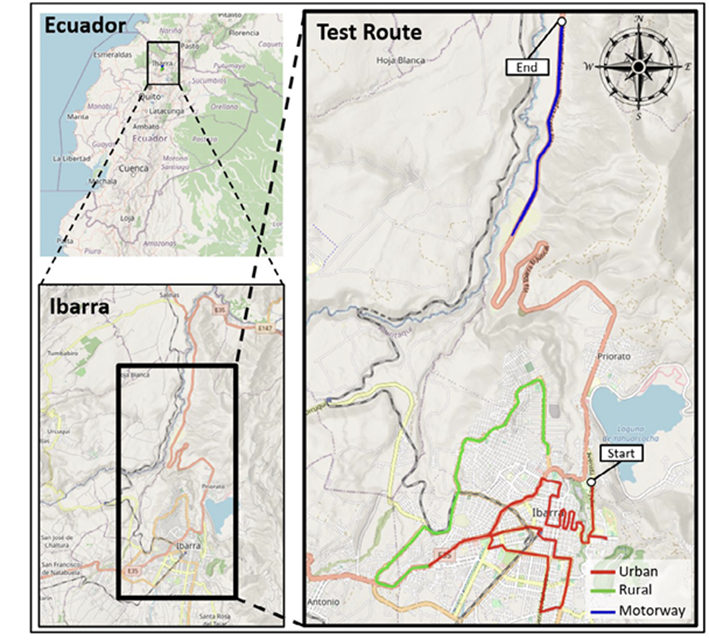
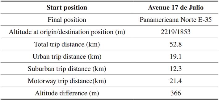
In this study, an experimental campaign was conducted along a test route designed in the city of Ibarra, Ecuador. This city is the capital of the province of Imbabura and has a population of approximately 200 000 inhabitants. In terms of vehicle fleet, Ibarra has experienced a significant growth of approximately 6 % per year in recent years⁽¹⁸⁾, which has generated challenges in terms of traffic and mobility. In this study, the test route was designed under the regulation (EU) 2017/1151⁽¹⁰⁾, which establishes different kinematic parameters, such as distance by route section, vehicle speeds, cumulative altitudes, and total trip duration. Hence, this study was carried out on an RDE test route (with approximately 53 km) including urban (0-60 km/h), suburban (60-90 km/h), and motorway (>90 km/h) sections, as shown inFig. 1. However, it is important to mention that this study is not intended to represent an RDE homologation process to evaluate the fuel consumption and CO₂emissions of the vehicle. In addition, details of the test route are provided inTable II.

Fig. 1 Selected experimental route for field data collection. 

Table II Information of Test Route 

C. Instrumentation

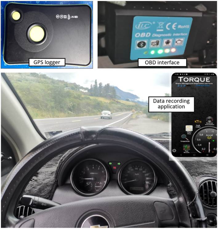
In general, the study required instruments for measuring the following three types of information: (I) vehicle kinematics (for example, position and speed), (II) vehicle and engine operating parameters (for example, torque and speed engine values), and (III) instantaneous fuel consumption data. A global positioning system (GPS) logger device, called ‘GL-770’, was installed in the test vehicle to record latitude, longitude, altitude, and vehicle speed with a frequency of 1Hz. It is important to note that this device is non-intrusive, resulting in the collection of vehicle kinematic information without affecting the regular operation of the tested vehicle operation. To record engine operating parameters and the vehicle fuel consumption data, an OBD interface device (called ELM Electronics 327) was connected to a mobile phone application (called Torque Pro). The ELM 327 was connected to the OBD2 diagnostic port to read the engine operating parameters in real time from the engine control unit (ECU). At the same time, these parameters were sent via Bluetooth from the ELM 327 to the Torque Pro mobile application to be recorded. In this study, the paid version of Torque Pro was used to set the 1 Hz sampling time of the data. The three instruments used for field data collection are shown infigure 2.

Fig. 2 Tested vehicle equipped on board with GPS logger, OBD interface, and OBD data recording application for field data collection. 

D. Experimental campaign

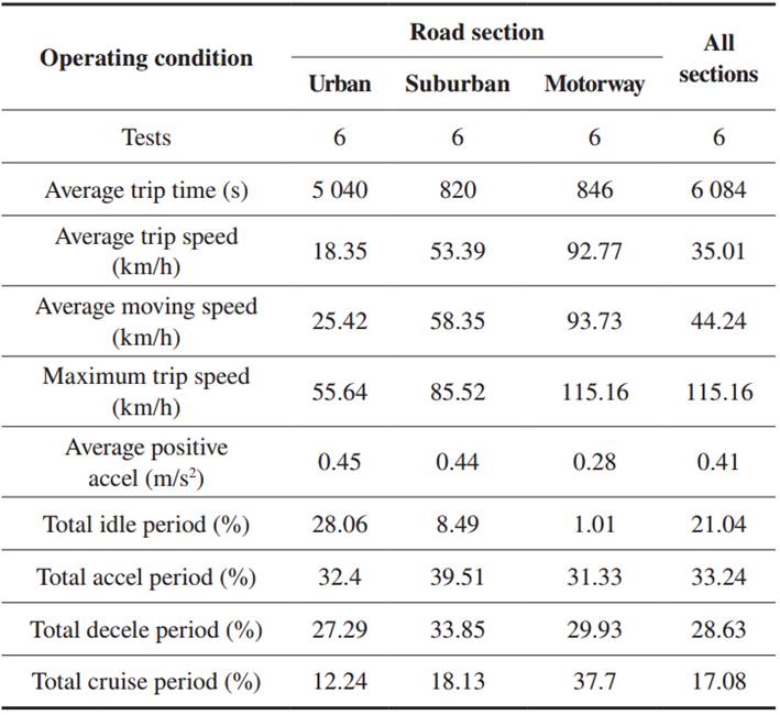
As mentioned above, a Chevrolet Aveo vehicle equipped with GPS and OBD interface devices was evaluated on a test route in the city of Ibarra. The experimental campaign of this study was conducted in February 2023. The campaign for the tested vehicle included both peak (7:00 and 13:00) and non-peak (10:00 and 15:00) periods. The vehicle was driven normally on the test route, respecting the traffic signals and speed limits established in the city. During the experimental campaign, the vehicle was powered by a commercially available type of gasoline called ‘Extra’ in Ecuador. This gasoline is characterised by an octane number of 85. The air conditioning of the vehicle was turned off to avoid additional loads on the engine operation during the experimental campaign. Before the start of each test, the vehicle was warmed up for 15 minutes until the engine reached normal operating temperature. To ensure the repeatability of the tests, the same driver drove the vehicle during all tests. Regarding the passenger load, the campaign was conducted with two people: a driver and a staff technician. The experimental campaign included six entire trips on the RDE route. These tests were conducted during peak periods (7:00 and 13:00) and off-peak periods (10:00 and 15:00). This strategy was designed to ensure that the results obtained accurately reflected vehicle performance at different levels of congestion. The average duration of each entire trip (urban, suburban and motorway road sections) on the test route was approximately 1.7 hours, and the average trip speed of the vehicle was approximately 35 km/h.Table IIIshows an overview of the operating conditions for the tested vehicle by road section in the experimental campaign.

Table III Overview of the operating conditions for the tested vehicle in terms of the road section in the experimental campaign 

E. Pre-processing real-world vehicle data

In this study, the applied preprocessing method was developed using R Studio software⁽¹⁹⁾. As the measurements of the experimental campaign were recorded using two devices with different initial recording times, a preprocessing step was developed to synchronise the different signals from the two devices through the vehicle speed. This speed was recorded second-by-second using both the GPS position data and through the OBD system of the vehicle. It is important to mention that the speed profiles were smoothed using a moving window filter⁽²⁰⁾. Overall, the data pre-processing stage ensures to guarantee of the results presented in this study.

F. Method for developing engine maps based on OBD data

Three variables are necessary in order to develop an engine map graph. Typically, torque and speed are used as the primary factors for the horizontal and vertical axes of the maps. Meanwhile, the third variable (Brake Thermal Efficiency (BTE), fuel consumption, brake-specific fuel consumption (BSFC) and emission rates) served as the parameter defining the theme of the map. In this study, the method applied to develop the engine maps included the following two stages: (1) generate grid engine maps by engine speed and torque ranges with averaged values of the third variable, and (2) develop two-dimensional contour engine maps based on grid data. These two stages were performed using R Studio⁽¹⁹⁾.

Initially, the grid engine maps were developed following the methodology proposed by Rosero et al.⁽²¹⁾. Initially, grids were generated based on torque and speed engine intervals, and the remaining engine operating data (referred to as the third variable) were assigned to their corresponding grid. Subsequently, the grouped data were averaged to obtain a single value by grid (speed-torque). Outliers were filtered by examining the relative frequency and standard deviation of each data group. Finally, the averaged values were discretized and assigned specific colours for each data interval when plotted on the engine maps.

Subsequently, to plot the two-dimensional contour engine maps, this study utilized the RStudio software⁽¹⁹⁾with an R package called ‘ggplot2’ R⁽²²⁾. This package includes a function named ‘geom_contour_filled()’, which generates contour plots using z variable observations (for example, fuel consumption, and emission rates) that should be previously grouped into interval combinations of two variables, x (engine speed) and y (torque). Based on this requirement, the data matrices resulting from the grid engine were used as input data to generate the contour engine maps. Finally, to develop the Contour-plot engine maps, a divergent colour scale was applied for each defined interval of the third variable. As a result of these two processing stages, this study obtained contour maps of BTE, BSFC, brake-specific CO₂emissions, fuel consumption rates and CO₂rates.

A. Effective power and torque of the engine

The OBD system provided engine load values ( L e obd ) as a percentage relative to the maximum effective power ( 𝑃 𝑒 𝑚𝑎𝑥 ) that the engine could produce. Based on the technical specifications of the tested vehicle manufacturer, the 𝑃 𝑒 𝑚𝑎𝑥 assumed for this study was 76 kW. To determine the actual effective engine power ( 𝑃 𝑒 ) in kW at any given moment, equation 1 was utilized.

The instantaneous engine torque values (𝜏) expressed in N.m, were calculated by multiplying the effective power and the engine speed.

B. Fuel energy efficiency and CO ₂ emission factors

The grid engine map generation process involved the calculation of the second-by-second BTE and BSFC values expressed in (%) and (𝑔/𝑘𝑊ℎ), respectively, for the tested engine. These calculations were performed using equation 2 and 3, as follows:

Here, 𝐹𝐶 is the instantaneous fuel consumption expressed in (g/s), ?? 𝑡ℎ represents the instantaneous thermal power (kW) resulting from the fuel being injected, while 𝐶 𝑉 𝑓𝑢𝑒𝑙 is the calorific value of the gasoline used (46.3 𝑀𝐽/𝑘𝑔)⁽²³⁾.

In this study, based on the stoichiometry of gasoline combustion, the CO₂emission rate (𝐸 𝑅 𝐶 𝑂 2 ) was calculated using equation 4 as follows:

Here, since the fuel utilized is gasoline (C₈H1₈), the assumed values were 18 for hydrogen (H) and 8 for carbon (C)⁽²⁴⁾.

To assess the performances of the tested engine for different road sections (𝑖), the average values of BTE (%), BSFC (g/kWh), energy-specific CO₂emission factor (g/kWh), as well as fuel consumption and CO₂emission rates (g/s), were estimated using equations 5, 6, 7, 8, 9, as follows:

Here, T is the number of second-by-second test data.

Moreover, to evaluate the vehicle performance for different road sections, the average distance-specific fuel consumption 𝐹𝐶 𝑑 and CO₂ emission 𝐸 𝐹 𝐶 𝑂 2 𝑑 factors, expressed in (g/km), were estimated using equations 10 and 11, as follows:

A. Typical engine operation patterns by torque and speed

Figure 3presents the patterns of engine operation by torque and speed for motorway, suburban, and urban roads. Grey circles represent the cumulative relative frequency (CRF) of engine operation points calculated for each torque and speed interval, while yellow shaded areas identify the highest engine operation patterns. In the case of the motorway section, the engine operated approximately 85 % of the time in a speed range of 2 500-3 500 rev/min, which are half-load intervals considering that the maximum engine power is reached at 5 800 rev/min. On the suburban section, engine performance was heterogeneous, operating approximately 95 % between low and high (75-100 N·m) torque ranges and low and medium (3 000-3 500 rev/min) speed ranges. In the case of the urban section, approximately 50 % of engine operation was between the lowest torque and lowest speed ranges. Based on Table II, these low-load operation results for urban roads are related to the fact that the vehicle operated with approximately 30 % at idle conditions and an average travel speed of less than 20 km/h. Overall, these results demonstrate that the type of road section significantly influences the torque and speed ranges that a vehicle engine can operate in real traffic conditions. This is consistent with that reported by Bishop et al.⁽²⁵⁾, who also found that the engine load patterns can vary with the type of road section, especially due to large changes in vehicle kinematics. In fact, Bishop et al. found that a light passenger vehicle engine ran approximately 35 % in low (90-110 N·m) torque ranges and low (1 000-1 500 rev/min) speed ranges. This value of 35 % operation at low load conditions is slightly higher than the 30 % found in the present study. Moreover, Tsiakmakis et al.⁽²⁶⁾reported that the average travel speed and 𝑣∗𝑎 factors for light passenger vehicles (LDVs) vary significantly with the type of road section. In fact, Tsiakmakis et al. found that between motorway and urban sections, the average trip speed was reduced approximately 3.5 times (from 67 to 19 km/h). Whereas, in the present study, this speed was strongly reduced by 5 times (from 92 to 18 km/h).

Fig. 3 Typical engine operation patterns by type of road section for all data points. 

B. Contour engine maps based on OBD data

1. Fuel energy efficiency and brake-specific CO2 emission maps

Figure 4illustrates the contour engine maps for BTE (a), BSFC (b), and brake-specific CO₂emissions (c). Infigure 4. a) the areas with the highest BTE (light green) values correspond to operating ranges with medium torque and engine speed, while those with the lowest efficiency (blue) are in areas of low torque demand. Additionally, at high torque and speed ranges, the engine shows values above 25 %. Infigure 4.b) and 4.c) it can be seen that the contours with the lowest fuel efficiency and brake-specific CO₂emissions (respectively) are in low torque ranges, which are common for an engine running in idle mode.Figure 4. b) shows that the largest contour corresponds to a range of BSFC with values between 175 and 250 g/kWh. This range is typical for engines mounted on light vehicles⁽²⁷⁾.Figure 4.c) shows that the lowest CO₂emissions (light green) areas with values below 600 g CO2/kWh are in the mid-range of torque and speeds. Overall, these results indicate that the lowest fuel consumption and CO₂emissions correspond to medium torque and engine speed ranges. Similar patterns were found by previous studies that evaluated engine performance of engines based on the engine mapping approach⁽¹³⁾,⁽²⁵⁾. In fact, Bishop et al.⁽¹³⁾found that between medium and high load conditions, the brake-specific CO2 emissions of an engine were reduced by approximately 2.5 times (from 500 to 200 g CO₂/kWh). Moreover, these three figures show that in idle mode, which is typical of urban operation conditions, the engine has a lower fuel efficiency in terms of energy.

Fig. 4 Engine maps for (a) brake thermal efficiency, (b) brake-specific fuel consumption, and (c) brake-specific CO2 emissions. 

2. Fuel consumption and emission rates maps

Figure 5.a) and 5.b) present contour engine maps for fuel consumption and CO₂emissions rates, respectively. Overall, these figures have similar sharply increasing trends (from light green to blue areas) of strong increase. In fact,Figure 5.a) and 5.b) show that the engine under maximum power operating conditions with an increase in torque and speed, fuel consumption and CO₂emissions rates reached the highest values (blue) of 3.5 and 10.0 g/s, respectively. In contrast, as expected, when there is a lower demand for engine power, the fuel consumption and emission rates have the lowest values (light green). Although these green areas show lower fuel consumption expressed in terms of rates, based on Figure 5, it can be stated that these same areas are the least efficient in energy terms. The resultant increasing trends are consistent with previous works for LDV’s⁽¹³⁾,⁽¹⁴⁾,⁽²⁸⁾and heavy-duty vehicles (HDV’s)⁽²¹⁾,⁽²⁹⁾, and emissions models⁽³⁰⁾. For instance, Mera et al.⁽¹³⁾found that between low and high load conditions, the CO₂emissions rates of an LDV engine increased approximately 20 times (from 0.32 to 7.2 g CO₂/s). Similarly, in the present study, the CO₂emissions rates were increased by about 14 times (from 0.69 to 10 g CO₂/s). It is important to note that the information contained infigure 5, expressed in terms of (g/s), can be used as input data to develop an empirical emission model. Previously, the information from the maps must be arranged in the form of a matrix by torque and engine speed intervals⁽²¹⁾,⁽³¹⁾. The model can predict second-by-second fuel consumption and CO₂emission values of the vehicle for any given operating scenario. Hence, future work will focus on using the engine map matrix resulting from this study for predicting fuel consumption and emissions of a vehicle by using torque and speed signals from engine operation as input data.

Fig. 5 Engine maps for (a) fuel consumption, and (c) CO2 rates. 

C. Overview of vehicle engine performance

Table IVshows the overall engine performance of the tested vehicle for motorway, suburban, and urban road sections. The performance of the vehicle is expressed in terms of energy-emission factors, average emission rates and distance-emission factors. In the case of BTE, the average value was 27 % for all sections, although in urban a BTE of approximately 25 % was found. This result is consistent withfigure 3and4, which showed that in urban conditions, the engine frequently ran in low torque and speed ranges, where there was lower fuel efficiency. In the case of energy-emission factors, this study found an average value of BSFC and CO₂of approximately 275 and 716 g/kWh, respectively. The minimum BSFC was for the motorway section with 250.18 g/kWh. In the case of the CO₂emission factor in terms of distance, the average value was approximately 190 g/km. Comparing urban and motorway road sections, CO₂emission factors of the vehicle increase by up to 50 %. The average value of 190 g CO₂/km found in the present study is higher than the range of 140-150 g CO₂/km reported by Zurita et al.⁽³²⁾, who used standardized driving cycles (for example, New European Driving Cycle (NEDC) and Federal Test Procedure (FTP) 75) to evaluate the performance of a Chevrolet Aveo under controlled laboratory conditions. This demonstrates the importance of a vehicle being evaluated with driving cycles that reflect the actual kinematic conditions of the spatial domain in which the vehicle operates⁽³³⁾. Otherwise, there may be a discrepancy between the values obtained in type-approval processes and those obtained in real traffic conditions. Overall, these results demonstrate that the vehicle and its engine performed better in highway conditions. Hence, to improve engine performance, especially in urban conditions, the use of start-stop technologies in engines is a valid strategy⁽²⁸⁾. This leads to reduced engine running times in low load ranges (idle conditions), which are characterized by low fuel efficiency as this study has shown.

Table IV Overall engine performance of fuel efficiency, energy emissions, emission rates, and distance emissions (from vehicle) by road section